

U  2.25             # Coulomb repulsion (F0)
mu 1.125            # Chemical potential
beta 100            # Inverse temperature
mode SM             # S stands for self-energy sampling, M stands for high frequency moment tail
M 5000000           # Number of Monte Carlo steps
svd_lmax 30         # number of SVD functions to project the solution
nom 80              # number of Matsubara frequency points to sample
tsample 200         # how often to record the measurements
aom 1               # number of frequency points to determin high frequency tail
GlobalFlip 1000000  # how often to perform global flip
Delta Delta.inp     # Input bath function hybridization
cix one_band.imp    # Input file with atomic state
Acceptance ratio: add/rm=0.2335 mv=0.545 number of accepted steps=1213234which means that adding or removing kinks had 23% success rate and moving kinks 54% success. If these numbers are high, it is advisable to have smaller t_sample.
This is the file that enumerates all atomic/cluster states, in the absence of the fermionic bath, and also contains the matrix elements of the creation operators. Hence, one needs to perform an exact diagonalization of the atom to run the ctqmc. Note that this can be very useful, as the same code can run not just the Hubbard type models, but also Kondo type models, without any modification.
We first show the cix file for the single band model, which is already included in the iterate.py script:
# cluster_size, number of states, number of baths, maximum matrix size
1 4 2 1
# baths, dimension, symmetry, global flip
0       1 0 0
1       1 0 0
# cluster energies for unique baths, eps[k]
0 0
#   N   K   Sz size F^{+,dn}, F^{+,up}, Ea  S
1   0   0    0   1   2         3        0   0
2   1   0 -0.5   1   0         4        0   0.5
3   1   0  0.5   1   4         0        0   0.5
4   2   0    0   1   0         0        0   0
# matrix elements
1  2  1  1    1    # start-state,end-state, dim1, dim2, <2|F^{+,dn}|1>
1  3  1  1    1    # start-state,end-state, dim1, dim2, <3|F^{+,up}|1>
2  0  0  0
2  4  1  1   -1    # start-state,end-state, dim1, dim2, <4|F^{+,up}|2>
3  4  1  1    1
3  0  0  0
4  0  0  0
4  0  0  0
HB2                # Hubbard-I is used to determine high-frequency
# UCoulomb : (m1,s1) (m2,s2) (m3,s2) (m4,s1)  Uc[m1,m2,m3,m4]
0 0 0 0 0.0
# number of operators needed
0
Comment lines are ignored by the code, but the code expects some string or empty line. The second line contains the cluster size (1 for single site), the number of all atomic states (which is 4 for a single impurity, i.e., empty site, spin down, spin up, and doubly occupied site). This is followed by the number of bath blocks, i.e., the type of bands that hybridize with the impurity. Here we have spin-up and spin-down bath, hence number of baths is 2. Finally, the second line specifies the maximum size of the matrix, which defines the electron creation operator. In general, it is larger than one, when we have full Coulomb interaction.
Following the third line, we have several lines, which specify the type of baths we have. Since we specified that there are two baths, we need to have here two lines, one for spin-up and one for spin-down. The first number in the line is just increasing integer, the second specifies the dimension of the bath block. Each block is one dimensional here. Next we specify which blocks are equivalent due to symmetry. Here we have paramagnetic state, hence the two baths have the same index. Finally, we have a number, which specifies which baths should be flipped by the global flip. Two baths, which have the same index, will be exchanged.
After a comment line, we have single line for each atomic state (more precisely block of atomic states). Since we have four atomic states, there are four lines. First number stands for the index, second for site occupancy, third for momentum (which is irrelevant here), then it is Sz of the atomic state. This is followed by the dimension of the block. After that, we have so-called index table.
The idea of the cix file is that we block together all atomic eigenstates, which are coupled by creation operators (this is explained in PRB 75:155113 (2007) ). Once we have all blocks enumerates, we can have an index table, which says that creation operator for spin-down changes atomic block state 1 to state state 2, and creation operator for spin-up changes atomic state 1 to state 3. We also see that atomic state 2, under the action of creation operator for up-spin, results in doubly-occupied site (state 4), and that applying creation operator for down-spin is not allowed (Pauli principle). Hence, these two columns (in general there are as many columns as there are creation operators in the problem) specify the index table.
Finally, there are two more numbers sets in each line. The first stand for the atomic energy, and the second for the total spin quantum number. Here the energy excludes the trivial term due to Coulomb repulsion F0 and the chemical potential shift mu. Inside ctqmc code, each atomic state energy will be added a term U*N*(N-1)/2.-mu*N, where U and mu are specified in the params file, and N is specified in the second column.
Now that we specified the index table for creation operator, we need to specify the matrix elements of the creation operators. The following eight lines specify such matrix elements. In general there are number-of-atomic-state*number-of-baths lines.
For each atomic state, there are two lines, because we have two baths. The first is for spin-down and the second for spin-up creation operator. Here we need to follow the order chosen above in the index table. The first number in each line stands for the state on which creation operator acts, and the second is the resulting state number. These numbers should match the index table. The next two numbers specify the dimension of the starting and the resulting block (here everything is one dimensional). For resulting states, which are not allowed by the Pauli principle, we just write 0 for dimension. Finally, we give the matrix element value. In general we would have here a matrix of dim1*dim2, where dim1 is the dimension of the starting state, and dim2 the resulting state.
The next few lines specify the high frequency tails. In this version of the code, the key word HB1 or HB2 must follow the matrix elements. This forces ctqmc to either use Hubbard-1 (HB1) or computes moments analytically (HB2). But which one is chosen, can now be specified through mode=M or H in the PARAMS file, which overwrites this settings.
If we want to calculate moments analytically, i.e., mode=M, we need to specify the tensor of Coulomb repulsion. We need to specify here only the non-zero values of the Coulomb repulsion. Each line means one non-zero value for the four dimensional tensor of the Coulomb repulsion. However, we choose to exclude the trivial F0 term, which can be added later inside ctqmc code. Hence, for the single orbital model, there is no Coulomb U beyond F0, hence we do not need to specify anything. We choose to add a single line of zeros. In general, we would have four integer numbers for the index of for orbitals, and one floating point number for the value of the Coulomb repulsion.
Finally, we can sample any number of equal time operators during the
run. The matrix elements of such operators would need to be specified
here. We decided not to sample any other operator.
Since the single-orbital model is perhaps to trivial, we will explain
also two other more complex examples. First, the two band model, and
next a plaquette with four sites, and a single orbital per site.
Let's start with the two band model, which can be downloaded here:
# Cix file for cluster DMFT with CTQMC
# cluster_size, number of states, number of baths
1 16 4 1
# baths, dimension, symmetry, global-flip
  0  1   0   0
  1  1   0   0
  2  1   1   1
  3  1   1   1
# cluster energies for unique baths, eps[k]
0 0
#   N   K   Sz size
1   0   0    0  1     2   5   3   4      0   0   # 00
2   1   0  0.5  1     0   6   7   8      0   0   # u0
3   1   0  0.5  1     7  10   0   9      0   0   # 0u
4   1   0 -0.5  1     8  11   9   0      0   0   # 0d
5   1   0 -0.5  1     6   0  10  11      0   0   # d0
6   2   0    0  1     0   0  12  13      0   0   # 20
7   2   0    1  1     0  12   0  14      0   0   # uu
8   2   0    0  1     0  13  14   0      0   0   # ud
9   2   0    0  1    14  15   0   0      0   0   # 02
10  2   0    0  1    12   0   0  15      0   0   # du
11  2   0   -1  1    13   0  15   0      0   0   # dd
12  3   0  0.5  1     0   0   0  16      0   0   # 2u
13  3   0 -0.5  1     0   0  16   0      0   0   # 2d
14  3   0  0.5  1     0  16   0   0      0   0   # u2
15  3   0 -0.5  1    16   0   0   0      0   0   # d2
16  4   0    0  1     0   0   0   0      0   0   # 22
# matrix elements
1   2    1 1       1
1   5    1 1       1
1   3    1 1       1
1   4    1 1       1
2   0    0 0
.....
.....
HB2
# UCoulomb : (m1,s1) (m2,s2) (m3,s2) (m4,s1)  Uc[m1,m2,m3,m4]
0  0  0  0    0
# number of operators needed
0
The four baths are all written in terms of a one dimensional blocks, and we assume that there is spin degeneracy, but the self-energy for the first orbital is different than for the second (symmetry index is different for the first two and the second two baths). Global flip exchanges the first two baths, and also the second two baths, since they have the same index.
We choose no crystal field splittings between the two baths, hence eps[k] is set to zero.Next we enumerate all states, and we give N, Sz, index table... for each state. After the comment, we also explain what each state stands for, for example up means the first orbital contains spin-up, and the second contains spin-down electron.
There are 16*4 lines of matrix elements, which we did not fully write
out. One can examine them in the attached file.
Finally, let us give example of a plaquette (four-site) DMFT problem,
with single orbital per-site. Here we need to perform the exact
diagonalization with a chosen U=F0, because the cluster eigenvectors
depend on the value of U, and the atomic state energies non-trivially
depend on U. Hence, in the PARAMS file we will set U=0, and we
will include U in the cix-file. We give here example for
U=6t, which is close to the Mott transition.
# Cix file for cluster DMFT with CTQMC
# cluster_size, number of states, number of baths, maximum_matrix_size
4 84 8 12
# baths, dimension, symmetry, global flip
0   1 0    0   # Sz=dn, K=(0,0)
1   1 0    0   # Sz=up, K=(0,0)
2   1 1    1   # Sz=dn, K=(pi,0)
3   1 1    1   # Sz=up, K=(pi,0)
4   1 1    2   # Sz=dn, K=(0,pi)
5   1 1    2   # Sz=up, K=(0,pi)
6   1 2    3   # Sz=dn, K=(pi,pi)
7   1 2    3   # Sz=up, K=(pi,pi)
# cluster energies for non-equivalent baths, eps[k]
-2 -0 2
 #   N   K   Sz size
 1   0   0    0   1      2   3   4   5   6   7   8   9                  0                  0
 2   1   0 -0.5   1      0  10  11  12  14  15  17  18                 -2                0.5
 3   1   0  0.5   1     10   0  12  13  15  16  18  19                 -2                0.5
 4   1   1 -0.5   1     11  12   0  10  17  18  14  15                  0                0.5
 5   1   1  0.5   1     12  13  10   0  18  19  15  16                  0                0.5
 6   1   2 -0.5   1     14  15  17  18   0  10  11  12                  0                0.5
 7   1   2  0.5   1     15  16  18  19  10   0  12  13                  0                0.5
 8   1   3 -0.5   1     17  18  14  15  11  12   0  10                  2                0.5
.......
# matrix elements
 1   2    1   1                     1
 1   3    1   1                     1
 1   4    1   1                     1
 1   5    1   1                     1
 1   6    1   1                     1
 1   7    1   1                     1
 1   8    1   1                     1
 1   9    1   1                     1
 2   0    0   0
 2  10    1   4        0.952550727929                    0       0.188982236505      -0.238606003712
 2  11    1   2                     1                    0
......
HB1
# number of operators needed
0
Here we choose to work in the basis with momentum as a good quantum number, and we will choose baths to be enumerate by momentum and spin. We commented for each bath how was it chosen. Note that in the input/output file for ctqmc, we will find the same order of baths. But in Delta.inp we will specify only baths, which are different. Since we have only four different baths, we will give only for baths in Delta.inp file.
In the section on matrix elements, we have states of dimension higher than one. In this case, we need to specify dim1*dim2 numbers in a single row.
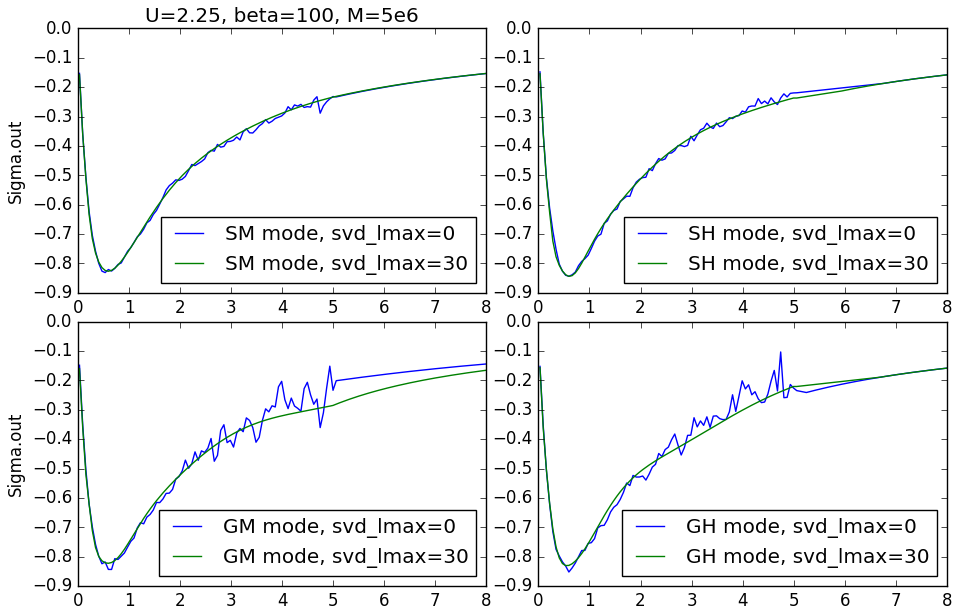
Finally, to perform the c-DMFT calculation for the Hubbard cluster, we give here an example of the python script iterate_cluster.py, which implements the DMFT self-consistency condition. To start, one also needs the cix-file hubbard_U_6_normal.cix. We also give the converged self-energy Sig.out, which should be the self-consistent solution at this U.
If one desires to calculate the cix file for other values of U,
we want to give the tarbal with cix-file
generator for the Hubbard model.
For good statistic, one should run the script on a parallel cluster
with a hundred cores or so. One should specify in "mpi_prefix.dat"
file, how should the parallel job be executed. For example "mpirun -n 100".
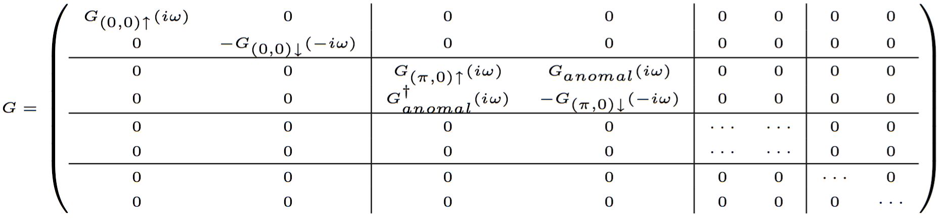
For completness we also mention more complicated example of d-wave
superconducting state in plaquette DMFT.
# Cix file for cluster DMFT with CTQMC
# cluster_size, number of states, number of baths, maximum_matrix_size
4 84 6 12
# baths, dimension, symmetry, global flip
  0   1       0                   0
  1   1     -0*                   1
  2   2       1    3    3  -1*    2
  3   2       1   -3   -3  -1*    3
  4   1       2                   4
  5   1     -2*                   5
# cluster energies for non-equivalent baths, eps[k]
-2 -0 2  0
 #   N   K   Sz size
 1   0   0    0   1      3   0   5   0   7   0   9   0                  0                  0
 2   1   0 -0.5   1     10   1  12   0  15   0  18   0                 -2                0.5
 3   1   0  0.5   1      0   0  13   0  16   0  19   0                 -2                0.5
 4   1   1 -0.5   1     12   0  10   1  18   0  15   0                  0                0.5
 5   1   1  0.5   1     13   0   0   0  19   0  16   0                  0                0.5
 6   1   2 -0.5   1     15   0  18   0  10   1  12   0                  0                0.5
 7   1   2  0.5   1     16   0  19   0   0   0  13   0                  0                0.5
 8   1   3 -0.5   1     18   0  15   0  12   0  10   1                  2                0.5
acceptance add/rm for orbital [0]=0.06132 acceptance  move  for orbital [0]=0.06653
acceptance add/rm for orbital [1]=0.06229 acceptance  move  for orbital [1]=0.06582
....
in ctqmc.log, which show how different is acceptance in different orbitals. To regulate how often a kink is tried in each bath, we can set BathProbability to be different for different orbitals/baths. For example, if we have two different orbitals, and the first has much better statistics than the second, we would set BathProbability to [1,2], so that the second bath will now be tried twice as often as the first bath.

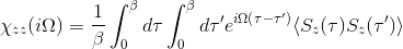

SampleSusc 1
We can also control the number of sampled bosonic frequencies by nomb parameter.
Notice that when susceptibility is sampled, we sample directly in Matsubara space and consequenctly switch svd_lmax=0.
The orbital susceptibility is a bit more challenging to sample, as it requires to apply an operator, which is not necessary commuting with the local Hamiltonian. We implemented the formula, which samples any susceptibility in the subspace spanned by the partition function. Notice that if the operator requires jumping between blocks of the local Hamiltonian (such as for example x or y component of the spin-susceptibility), it is likely nonzero in the space outside the configuration space of the partition function, and then this implementation would give wrong answer. One would need to use the worm algorithm to sample a general susceptibility. If the susceptibility corresponding to an operator O is nonzero only in the configuration space of the partition function, we can compute


# number of operators needed
# number of operators needed
 1
# number of operators needed
 1  1
The easiest way to use this feature is to run atom_d.py script, which performs exact diagonalization of the atom. We first prepare a file, which we call Trans.dat, that specifies the connection between the spherical harmonics and the orbitals used in ctqmc. Lets assume Trans.dat takes the form:
5 5 #  size of Sigind and CF
#---- Sigind follows
  1    0    0    0    0
  0    2    0    0    0
  0    0    3    0    0
  0    0    0    4    0
  0    0    0    0    5
#---- CF follows
  0.00000000   0.00000000    0.00000000   0.00000000    1.00000000   0.00000000    0.00000000   0.00000000    0.00000000   0.00000000
  0.70710679   0.00000000    0.00000000   0.00000000    0.00000000   0.00000000    0.00000000   0.00000000    0.70710679   0.00000000
  0.00000000   0.00000000    0.70710679   0.00000000    0.00000000   0.00000000   -0.70710679   0.00000000    0.00000000   0.00000000
  0.00000000   0.00000000    0.00000000   0.70710679    0.00000000   0.00000000    0.00000000   0.70710679    0.00000000   0.00000000
 -0.00000000  -0.70710679    0.00000000   0.00000000    0.00000000   0.00000000    0.00000000   0.00000000    0.00000000   0.70710679
Next we can execute
atom_d.py J=0.8 l=2 OCA_G=False "CoulombF='Full'" "Eimp=[0.0,-0.1,-0.02,-0.02,-0.06]" "ORB=[0,0,1,-1,0,0,0,1,-1,0]"


SampleSusc 1