Home What is? Install Overview CTQMC MnO FeSe SrVO3 LaVO3 Cerium Sr2IrO4 Ta2NiSe5 phonon

Tutorial 4: LaVO₃

Next example is on a correlated Mott insulator with a small gap LaVO₃. Its crystal structure contains 4-V atoms in the unit cell, which are in V³⁺ state, hence V ion has formally two electrons in d-shell. We will use DMFT for the electrons in the t_2g shell.

In the first step, DFT has to be converged to obtain a good charge density. Copy the LaVO3.struct file: This file contains the details of the crystal structure in the format that Wien2K uses. Initialize the DFT calculation by using init_lapw and then choose standard setting "0, a, 2, a, c, c, c, -up, 13, -6, c, 100, 1, c, n" respectively. These are pretty much the default values that Wien2K uses. We chose to work with the PBE functional, and use a shifted k-point grid of 100 points (in the whole Brillouin zone). Note that spin-orbit interaction can be safely ignored as there are no heavy ions in the system. Run the DFT calculation using the command "run_lapw".

In DMFT calculation, one needs converged frequency dependent local Green's function, hence more k-points is typically needed. We will increase the number of k-points to 500 in this tutorial. Note that the unit cell here is quite large, hence 500 points is not small. Run x kgen and specify 500 k-points with shifted k-mesh. Next, rerun wien2k on this k-mesh, i.e., run_lapw.

Once the DFT calculation is done, we have a good charge density to start a DMFT calculation. The next step is to initialize the DMFT calculation. For this, use the script "init_dmft.py" and choose the options:

Specify correlated atoms (ex: 1-4,7,8): 1-4

We choose all 4-V atoms as correlated.

   
For each atom, specify correlated orbital(s) (ex: d,f):
  1 V  3+: d
  2 V  3+: d
  3 V  3+: d
  4 V  3+: d

The partially filled d shell of the V ions is to be treated in DMFT.

Specify qsplit for each correlated orbital (default = 0):
    Qsplit  Description
------  ------------------------------------------------------------
     0  average GF, non-correlated
     1  |j,mj> basis, no symmetry, except time reversal (-jz=jz)
    -1  |j,mj> basis, no symmetry, not even time reversal (-jz=jz)
     2  real harmonics basis, no symmetry, except spin (up=dn)
    -2  real harmonics basis, no symmetry, not even spin (up=dn)
     3  t2g orbitals 
    -3  eg orbitals
     4  |j,mj>, only l-1/2 and l+1/2
     5  axial symmetry in real harmonics
     6  hexagonal symmetry in real harmonics
     7  cubic symmetry in real harmonics
     8  axial symmetry in real harmonics, up different than down
     9  hexagonal symmetry in real harmonics, up different than down
    10  cubic symmetry in real harmonics, up different then down
    11  |j,mj> basis, non-zero off diagonal elements
    12  real harmonics, non-zero off diagonal elements
    13  J_eff=1/2 basis for 5d ions, non-magnetic with symmetry
    14  J_eff=1/2 basis for 5d ions, no symmetry
------  ------------------------------------------------------------
  1  V  3+-1 d: 3
  2  V  3+-2 d: 3
  3  V  3+-3 d: 3
  4  V  3+-4 d: 3

This chooses the basis to use for the DMFT calculation. We will again choose to correlated the t_2g subshell only, which will save some time.

Specify projector type (default = 2):
  Projector  Drscription
------  ------------------------------------------------------------
     1  projection to the solution of Dirac equation (to the head)
     2  projection to the Dirac solution, its energy derivative, 
          LO orbital, as described by P2 in PRB 81, 195107 (2010)
     4  similar to projector-2, but takes fixed number of bands in
          some energy range, even when chemical potential and 
          MT-zero moves (folows band with certain index)
     5  fixed projector, which is written to projectorw.dat. You can
        generate projectorw.dat with the tool wavef.py
------  ------------------------------------------------------------

> 5

Do you want to group any of these orbitals into cluster-DMFT problems? (y/n): n

We do not attempt to do a cluster-DMFT calculation at this stage.

```
Enter the correlated problems forming each unique correlated
problem, separated by spaces (ex: 1,3 2,4 5-8): 1-4
```
All four V-atoms are equivalent, when described in their proper local coordinate system, hence we will be solving only one impurity problem.

Range (in eV) of hybridization taken into account in impurity
problems; default -10.0, 10.0:

We will again take the default -10,10 eV range.

```
Perform calculation on real; or imaginary axis? (r/i): r
      
```
We will first choose real axis, because we will need to find proper rotations to local coordinate system, and we want to plot DOS to see splitting of t_2g-e_g states.
```
Is this a spin-orbit run? (y/n): n
```
The spin-orbit coupling is ignored.

The init_dmft.py script generates the two DMFT input files, case.indmfl and case.indmfi, which connect the solid and the impurity with the DMFT egine, respectively. Let us take a closer look at the header of the file. This time it is more complex, containing 4 correlated atoms:

45 156 1 5                            # hybridization band index nemin and nemax, renormalize for interstitials, projection type
0 0.025 0.025 200 -3.000000 1.000000  # matsubara, broadening-corr, broadening-noncorr, nomega, omega_min, omega_max (in eV)
4                                     # number of correlated atoms
1     1   0                           # iatom, nL, locrot
  2   3   1                           # L, qsplit, cix
2     1   0                           # iatom, nL, locrot
  2   3   2                           # L, qsplit, cix
3     1   0                           # iatom, nL, locrot
  2   3   3                           # L, qsplit, cix
4     1   0                           # iatom, nL, locrot
  2   3   4                           # L, qsplit, cix

The first line specifies the hybridization window "(-10eV,10eV)" which contains bands with index 45-156. The projector type is 5. The number 1 in the middle stands for normalization of the projector. When performing self-consistent DMFT, we need to make sure that the Green's function is properly normalized (integral of the imaginary part is -pi). For plotting DOS, it is sometimes desired to remove this normalization, and use projector, which is normalized in band basis (not in orbital basis).

The second line contains a switch for the real-axis or imaginary axis calculation. For ctqmc impurity solver, we need to set "matsubara" to 1. The next two numbers specify the broadening in k-point summation. The last three numbers are used for plotting the spectral functions, to which we will return latter.

The third line specifies the number of correlated atoms, which is here 4, i.e., all V-atoms in the unit cell.

The next eigth lines can be grouped into set of 4 x 2, i.e., for each correlated V atom two lines. The first line in the group specifies the consequitive atom number (from case.struct), which we treat as correlated. It also specifies how many orbital indeces (different L's) we will use for projection (only 1). The last index "locrot" is used for rotation of local axis, and will be used it shortly, to specify the local coordinate system for DMFT basis.

The second line in a group specifies orbital momentum "l=2", "qsplit=3" which we choose during initialization. Each correlated orbital-set gets a unique index (correlated index) during initialization. These 4 blocks are enumerated by consecutive numbers cix=1,2,3,4. For each of these 4 correlated sets, a more detailed specification is given in the remaining of "case.indmfl" file.

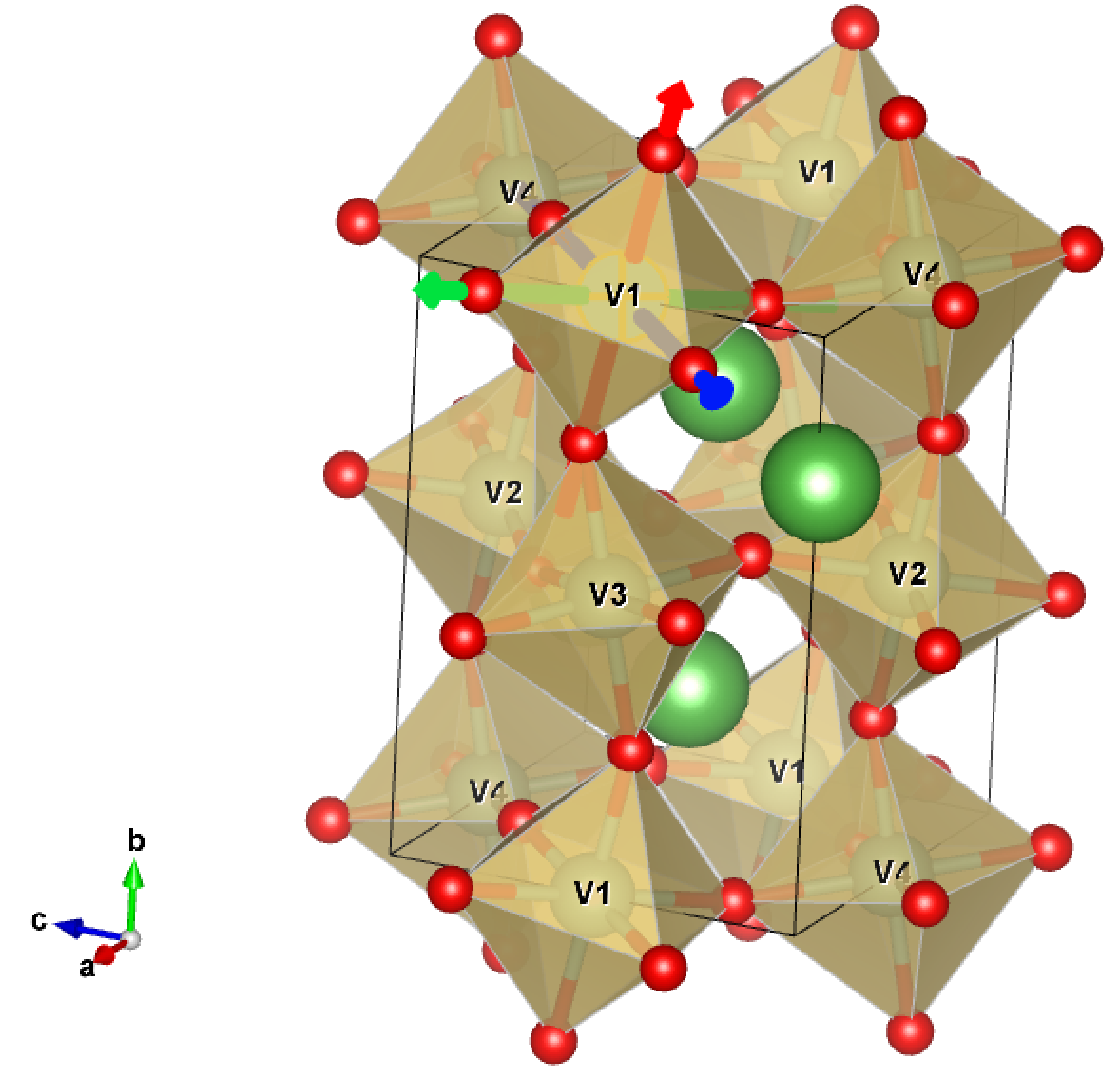
The global axis of the structure is not convenient for DMFT calculation. While in principle the DMFT is rotationally invariant method, and any axis should give the same result, in practice there is enormous difference in the severity of the quamtum Monte Carlo sign problem. To reduce/avoid sign problem, we always pick the local axis on each atom so that the hybridization matrix is maximally diagonal. This is usually the local axis, which is aligned with the local environment of the correlated atom, in this case octahedron. In this figure, we show how the local axis on V₁ will be choosen below.

In the binary directory, we have a tool to find such local coordinate axis. The script is

localaxes.py

Execute it when in directory with DFT calculation. The following are questions the script will ask:

  1 ATOM:  1  EQUIV.  1  V  3+      AT   0.00000   0.00000   0.50000
  2 ATOM:  1  EQUIV.  2  V  3+      AT   0.50000   0.50000   0.00000
  3 ATOM:  1  EQUIV.  3  V  3+      AT   0.00000   0.50000   0.50000
  4 ATOM:  1  EQUIV.  4  V  3+      AT   0.50000   0.00000   0.00000
......
Enter the atom for which you want to determine local axes: 1

Once you enter the index to first atom, you should get

trying  cube : -N= -2.000045418 chi2= 0.0781099540504 = 3.78604380855 combined-criteria 5.54201036661
trying  octahedra : -N= -4.55779706225e-05 chi2= 0.000198898591793 = 3.78604379544 combined-criteria 0.00392610291121
trying  tetrahedra : -N= -2.31787341618e-05 chi2= 0.582093832999 = 3.78514737663 combined-criteria 11.4900717126
trying  square-piramid : -N= -3.66084575019e-05 chi2= 0.493633610179 = 3.78568492083 combined-criteria 9.74393690443
According to angle variance and bond-angle we are trying octahedra with = 4.55779706225e-05 and = 0.000198898591793
Found the environment is ('octahedra', 4.5577970622545649e-05, 0.00019889859179304857)

Rotation to input into case.indmfl by locrot=-1 : 

  0.79186901   0.14777288   0.59254253 
 -0.03062084   0.97866938  -0.20314676 
 -0.60992282   0.14272147   0.77950288

The code figured out that we have octahedra, and it found the best axis for local coordinate system in cartesian coordinates.

Let us first understand this transformation matrix. It is a unitary transformation from global cartesian coordinate system to local cartesian coordinate system. New x-axis, y-axis and z-axis are given in the first, the second and the third row. One can plot these vectors in VESTA to visualize our choice. The matrix is not written in lattice coordinates, but cartesian coordinates. If one wants the same transformation in lattice coordinates, one needs to build a transformation from cartesian to lattice coordinates. There are several ways to do that. One can look at LaVO3.outputkgen, and find R1,R2,R3 at the top of the file

  R1 =  10.498336  0.000000  0.000000
  R2 =   0.000000 14.831856  0.000000
  R3 =   0.000000  0.000000 10.494575

The same information exists also in LaVO3.outputd under BR1_DIR. The transformation from cartesian to lattice coordinates is: C2L = Inverse([[R1x,R2x,R3x],[R1y,R2y,R3y],[R1z,R2z,R3z]]) which is here

0.0952532 0.0000000 0.0000000
0.0000000 0.0674224 0.0000000
0.0000000 0.0000000 0.0952873

hence new x-axis in lattice coordinates is C2L*(new-x) = (-0.00291502, 0.0659845, -0.0193558), etc. An alternative way to find transformation from cartesian to lattice coordinates is to inspect case.rotl (which appears after dmft1 is being run) at the top of the file one finds

 BR1
   0.59849   0.00000   0.00000
  -0.00000   0.42363   0.00000
  -0.00000  -0.00000   0.59871

It turns out that C2L = BR1/(2*pi).

Now that we have the transformation matrix to local coordinate system, we will add it to LaVO3.indmfl file. We will change locrot to -1 for the relevant atom, and paste below the transformation for that atom. The result for the first atom looks like that

  
1     1  -1                            # iatom, nL, locrot
  2   3   1                            # L, qsplit, cix
  0.79186901   0.14777288   0.59254253
 -0.03062084   0.97866938  -0.20314676
 -0.60992282   0.14272147   0.77950288

The set of atoms, which are equivalent in case.struct file, should use the same transformation to local axis. The reason is that the code will automatically find extra symmetry operation transforming first atom to any equivalent atom, and will add this extra transformation. If two or more atoms, which are not equivalent in structure file (they are not grouped together in case.struct file), are treated as correlated, one needs to find correct transformation (for example using script localaxes.py) for each of these inequivalent atoms.
The header of the LaVO3.struct file finally looks like that

45 156 1 5                            # hybridization band index nemin and nemax, renormalize for interstitials, projection type
0 0.025 0.025 200 -3.000000 1.000000  # matsubara, broadening-corr, broadening-noncorr, nomega, omega_min, omega_max (in eV)
4                                     # number of correlated atoms
1     1  -1                           # iatom, nL, locrot
  2   3   1                           # L, qsplit, cix
  0.79186901   0.14777288   0.59254253
 -0.03062084   0.97866938  -0.20314676
 -0.60992282   0.14272147   0.77950288
2     1  -1                           # iatom, nL, locrot
  2   3   2                           # L, qsplit, cix
  0.79186901   0.14777288   0.59254253
 -0.03062084   0.97866938  -0.20314676
 -0.60992282   0.14272147   0.77950288
3     1  -1                           # iatom, nL, locrot
  2   3   3                           # L, qsplit, cix
  0.79186901   0.14777288   0.59254253
 -0.03062084   0.97866938  -0.20314676
 -0.60992282   0.14272147   0.77950288
4     1  -1                           # iatom, nL, locrot
  2   3   4                           # L, qsplit, cix
  0.79186901   0.14777288   0.59254253
 -0.03062084   0.97866938  -0.20314676
 -0.60992282   0.14272147   0.77950288

The specification of correlated set is given in the second part of case.indmfl, which we did not change.

We next create a blank self-energy file to plot the Green's function in the new local coordinate system. We just execute

szero.py

Notice that the generated self-energy is now given on the real axis, because matsubara flag is set to 0.

Next we will run

x_dmft.py lapw1
x_dmft.py dmft1

which should produce LaVO3.cdos and LaVO3.gc[1-4]. Of course these should be compatible with the DFT densities of states.

If you wish to run these runs in parallel, you just need to specify mpi_prefix.dat file, which must contain the mpi_run command.

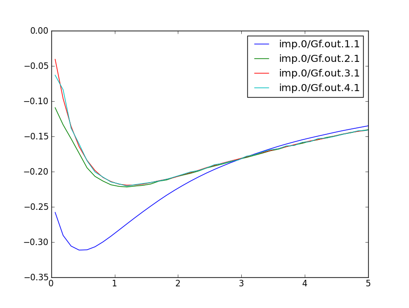
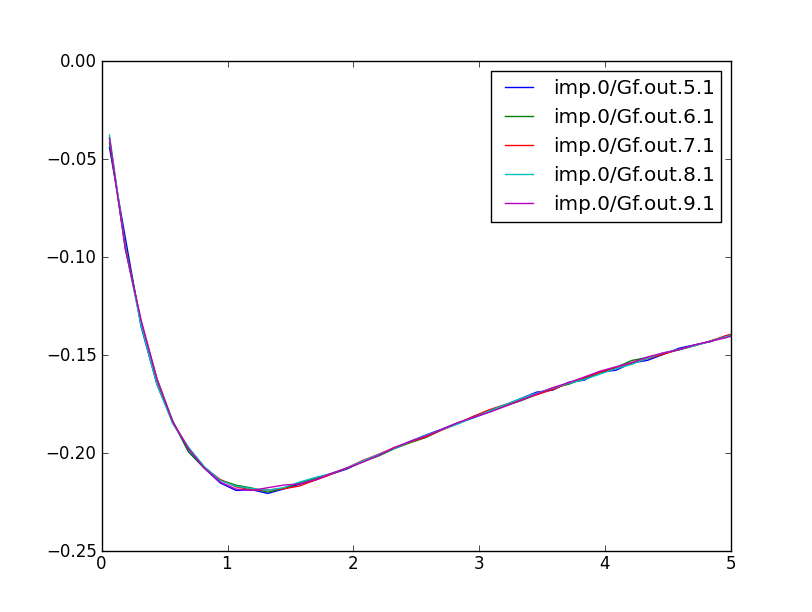
We can examine LaVO3.gc[1-4] which should all contain almost identical Green's function, which proves that the transformation between the four equivalent atoms was properly chosen. Next we realize that there is a splitting between the t_2g orbitals, and we will choose a local transformation, which will make hybridization as diagonal as possible. To do that, we first examine LaVO3.outputdmf1 file, which contains (towards the end) the following lines

 Full matrix of impurity levels follows
 icix=           1
   -0.01624121     0.00000000      -0.00712563     0.00000000      -0.01627386     0.00000000   
   -0.00712563    -0.00000000      -0.01061912    -0.00000000       0.01733578    -0.00000000   
   -0.01627386    -0.00000000       0.01733578     0.00000000      -0.02757288     0.00000000   
 
 icix=           1 at omega=0
    0.24430529     0.00000000       0.01913794     0.00000000       0.00245632     0.00000000   
    0.01913794    -0.00000000       0.26547163    -0.00000000      -0.03205887     0.00000000   
    0.00245632    -0.00000000      -0.03205887    -0.00000000       0.25124493     0.00000000

The first matrix specifies the impurity levels at infinite frequency, and the second matrix specifies the sum of the impurity levels and the hybridization matrix at zero frequency. The off-diagonal terms are only of the order of 20meV, which is very small compared to the gap. Nevertheless, we can transform to a better basis for our impurity solver. There are two ways to do that, i.e., automatically with the script findRot.py, or in a few steps explained below. As the script findRot.py is quite new, we will explain all the steps it performs.

Obtaining transformation by findRot.py

When using this script, we just type

findRot.py

in the directory where the impurity levels are available, and the script will copy the old LaVO3.indmfl file to LaVO3.indmfl_findRot and create a new version of it. You can test it by once more executing

x_dmft.py dmft1

and than checking that the impurity levels in LaVO3.outputdmf1 are diagonal. If you choose to use findRot.py, then you can jump to section on The rest of initialization

Obtaining transformation by a series of steps

We first prepare a text file, which contains the matrix of impurity levels from LaVO3.outputdmf1, and also the current transformation from spherical to cubic harmonics, which is specified in LaVO3.indmfl file. We will create a python text rot.dat file, which will contain the impurity levels in strHc variable and the transformation in strT2C variable:

strHc="""
 0.24430529    -0.00000000       0.01913794     0.00000000       0.00245632    -0.00000000
 0.01913794    -0.00000000       0.26547163    -0.00000000      -0.03205887     0.00000000
 0.00245632     0.00000000      -0.03205887    -0.00000000       0.25124493    -0.00000000
"""
strT2C="""
 0.00000000  0.00000000    0.70710679  0.00000000    0.00000000  0.00000000   -0.70710679  0.00000000    0.00000000  0.00000000
 0.00000000  0.00000000    0.00000000  0.70710679    0.00000000  0.00000000    0.00000000  0.70710679    0.00000000  0.00000000
-0.00000000 -0.70710679    0.00000000  0.00000000    0.00000000  0.00000000    0.00000000  0.00000000    0.00000000  0.70710679
"""

Then we run

find3dRotation.py rot.dat

and the script gives us new set of optimized orbitals:

:SUCCESS For orbital [0] the final transformation is real
:SUCCESS For orbital [1] the final transformation is real
:SUCCESS For orbital [2] the final transformation is real

Rotation to input : 
 0.00000000  0.43702058    0.34959590 -0.43219872    0.00000000  0.00000000   -0.34959590 -0.43219872    0.00000000 -0.43702058  
 0.00000000 -0.39025811    0.58445888  0.07814369    0.00000000  0.00000000   -0.58445888  0.07814369    0.00000000  0.39025811  
 0.00000000 -0.39586820   -0.19023811 -0.55416409    0.00000000  0.00000000    0.19023811 -0.55416409    0.00000000  0.39586820

We then copy these three new orbitals into LaVO3.indmfl file to replace the old three t2g orbitals in the Transformation matrix. Notice that this transformation matrix transforms from spheric harmonics to the new DMFT basis, and shows how these orbitals are defined. The columns correspond to the following quantum numbers (m_l=-2,-1,0,1,2). In the original transformation found in LaVO3.indmfl the rows correspond to ('xz','yz','xy','z^2','x^2-y^2'). Now we have a mixture of 'xz','yz' and 'xy' orbitals.

After the replacement of transformation matrices, the file LaVO3.indmfl contains:

#================ # Siginds and crystal-field transformations for correlated orbitals ================
4     5   3       # Number of independent kcix blocks, max dimension, max num-independent-components
1     5   3       # cix-num, dimension, num-independent-components
#---------------- # Independent components are --------------
'xz' 'yz' 'xy'
#---------------- # Sigind follows --------------------------
1 0 0 0 0
0 2 0 0 0
0 0 3 0 0
0 0 0 0 0
0 0 0 0 0
#---------------- # Transformation matrix follows -----------
 0.00000000  0.43702058    0.34959590 -0.43219872    0.00000000  0.00000000   -0.34959590 -0.43219872    0.00000000 -0.43702058
 0.00000000 -0.39025811    0.58445888  0.07814369    0.00000000  0.00000000   -0.58445888  0.07814369    0.00000000  0.39025811
 0.00000000 -0.39586820   -0.19023811 -0.55416409    0.00000000  0.00000000    0.19023811 -0.55416409    0.00000000  0.39586820
 0.00000000  0.00000000    0.00000000  0.00000000    1.00000000  0.00000000    0.00000000  0.00000000    0.00000000  0.00000000
 0.70710679  0.00000000    0.00000000  0.00000000    0.00000000  0.00000000    0.00000000  0.00000000    0.70710679  0.00000000
2     5   3       # cix-num, dimension, num-independent-components
#---------------- # Independent components are --------------
'xz' 'yz' 'xy'
#---------------- # Sigind follows --------------------------
1 0 0 0 0
0 2 0 0 0
0 0 3 0 0
0 0 0 0 0
0 0 0 0 0
#---------------- # Transformation matrix follows -----------
 0.00000000  0.43702058    0.34959590 -0.43219872    0.00000000  0.00000000   -0.34959590 -0.43219872    0.00000000 -0.43702058
 0.00000000 -0.39025811    0.58445888  0.07814369    0.00000000  0.00000000   -0.58445888  0.07814369    0.00000000  0.39025811
 0.00000000 -0.39586820   -0.19023811 -0.55416409    0.00000000  0.00000000    0.19023811 -0.55416409    0.00000000  0.39586820
 0.00000000  0.00000000    0.00000000  0.00000000    1.00000000  0.00000000    0.00000000  0.00000000    0.00000000  0.00000000
 0.70710679  0.00000000    0.00000000  0.00000000    0.00000000  0.00000000    0.00000000  0.00000000    0.70710679  0.00000000
3     5   3       # cix-num, dimension, num-independent-components
#---------------- # Independent components are --------------
'xz' 'yz' 'xy'
#---------------- # Sigind follows --------------------------
1 0 0 0 0
0 2 0 0 0
0 0 3 0 0
0 0 0 0 0
0 0 0 0 0
#---------------- # Transformation matrix follows -----------
 0.00000000  0.43702058    0.34959590 -0.43219872    0.00000000  0.00000000   -0.34959590 -0.43219872    0.00000000 -0.43702058
 0.00000000 -0.39025811    0.58445888  0.07814369    0.00000000  0.00000000   -0.58445888  0.07814369    0.00000000  0.39025811
 0.00000000 -0.39586820   -0.19023811 -0.55416409    0.00000000  0.00000000    0.19023811 -0.55416409    0.00000000  0.39586820
 0.00000000  0.00000000    0.00000000  0.00000000    1.00000000  0.00000000    0.00000000  0.00000000    0.00000000  0.00000000
 0.70710679  0.00000000    0.00000000  0.00000000    0.00000000  0.00000000    0.00000000  0.00000000    0.70710679  0.00000000
4     5   3       # cix-num, dimension, num-independent-components
#---------------- # Independent components are --------------
'xz' 'yz' 'xy'
#---------------- # Sigind follows --------------------------
1 0 0 0 0
0 2 0 0 0
0 0 3 0 0
0 0 0 0 0
0 0 0 0 0
#---------------- # Transformation matrix follows -----------
 0.00000000  0.43702058    0.34959590 -0.43219872    0.00000000  0.00000000   -0.34959590 -0.43219872    0.00000000 -0.43702058
 0.00000000 -0.39025811    0.58445888  0.07814369    0.00000000  0.00000000   -0.58445888  0.07814369    0.00000000  0.39025811
 0.00000000 -0.39586820   -0.19023811 -0.55416409    0.00000000  0.00000000    0.19023811 -0.55416409    0.00000000  0.39586820
 0.00000000  0.00000000    0.00000000  0.00000000    1.00000000  0.00000000    0.00000000  0.00000000    0.00000000  0.00000000
 0.70710679  0.00000000    0.00000000  0.00000000    0.00000000  0.00000000    0.00000000  0.00000000    0.70710679  0.00000000

We now rerun the dmft1 step

x_dmft.py dmft1

and check the new impurity levels. We find

 Full matrix of impurity levels follows
 icix=           1
    0.00888017    -0.00000000       0.00353679     0.00000000       0.00345745     0.00000000   
    0.00353679    -0.00000000      -0.03365887     0.00000000      -0.01070044    -0.00000000   
    0.00345745    -0.00000000      -0.01070044     0.00000000      -0.02965450     0.00000000   
 
 icix=           1 at omega=0
    0.21757484    -0.00000000      -0.00000000    -0.00000000      -0.00000000    -0.00000000   
   -0.00000000     0.00000000       0.24850424     0.00000000      -0.00000000    -0.00000000   
   -0.00000000     0.00000000      -0.00000000     0.00000000       0.29494278     0.00000000

which shows that at zero frequency we have completely diagonal hybridization, and also at infinity, the hybridization is much closer to diagonal then before.

The rest of initialization

Finally, DMFT initialization produced a second file, named case.indmfi, which contains the following lines:

1   # number of sigind blocks
5   # dimension of this sigind block
1 0 0 0 0
0 2 0 0 0
0 0 3 0 0
0 0 0 0 0
0 0 0 0 0

This specifies that we have only one quantum impurity problem to run, although there are four V-atoms in the unit cell. We transformed Green's functions to local basis, and hence all four V-atoms are equivalent in paramagnetic state. We do not need to change this file.

Next create a new folder, and when in that folder, use the command

dmft_copy.py <lda_results_directory>

where <lda_results_directory> is the directory where the output of the DFT calculation with DMFT initialization is. This command copies the necessary files to start a DMFT calculation. These include the .struct file as well as the various Wien2K input files such as .inm, .in1, etc. The charge density file, .clmsum, is also copied. This is all we need from the initial Wien2K run, and now we proceed to create the rest of the files, needed by the DMFT calculation.

There are a few more steps we need to to:

Next, edit LaVO3.indmfl and change the flag matsubara in second line from 0 to 1, because the impurity solver works on imaginary axis.
delete sig.inp file, which is given on real axis.
run szero.py to create a blank self-energy on imaginary axis.

copy params.dat file into working directory, which contains

solver         =  'CTQMC'   # impurity solver
DCs            =  'nominal' # double counting scheme

max_dmft_iterations = 3     # number of iteration of the dmft-loop only
max_lda_iterations  = 100   # number of iteration of the LDA-loop only
finish              =  30   # number of iterations of full charge loop (1 = no charge self-consistency)

ntail          =  300       # on imaginary axis, number of points in the tail of the logarithmic mesh

cc             =  5e-5      # the charge density precision to stop the LDA+DMFT run
ec             =  5e-5      # the energy precision to stop the LDA+DMFT run

recomputeEF    =  0         # Recompute EF in dmft2 step.

# Impurity problem number 0
iparams0={"exe"                : ["ctqmc"              , "# Name of the executable"],
          "U"                  : [6.0                  , "# Coulomb repulsion (F0)"],
          "J"                  : [0.8                  , "# Coulomb repulsion (F0)"],
          "beta"               : [50                   , "# Inverse temperature"],
          "CoulombF"           : ["'Ising'"            , "# Form of Coulomb repulsion"],
          "svd_lmax"           : [25                   , "# We will use SVD basis to expand G, with this cutoff"],
          "M"                  : [10e6                 , "# Total number of Monte Carlo steps"],
          "mode"               : ["SH"                 , "# We will use self-energy sampling, and Hubbard I tail"],
          "nom"                : [200                  , "# Number of Matsubara frequency points sampled"],
          "tsample"            : [200                  , "# How often to record measurements"],
          "GlobalFlip"         : [1000000              , "# How often to try a global flip"],
          "warmup"             : [1e6                  , "# Warmup number of QMC steps"],
          "nf0"                : [2                    , "# Double counting parameter"],
}

and is basically the same as in previous tutorials. The only difference is that nominal valence is here 2.0, and we will not recompute the chemical potential, as we expect a Mott-gap. We need to be careful that the solid is neutral (charge density is correct) by examining :DRHO in LaVO3.scf or the tail of dmft2_info.out. Note that at the beginning, some mismatch of charge is acceptable, but not once the charge is converged, :DRHO should be very small.

We notice that DCs='exactd' gives almost identical results. It is not surprising that dielectric screening is most appropriate for insulator like LaVO₃.

Now we are ready to run DFT+DMFT calculation. As in previous tutorial, you should set-up mpi_prefix.dat, which contains the command for running mpi job on your computer, for example
echo "mpirun -np $NSLOTS" > mpi_prefix.dat
or
echo "mpiexec -port $port -np $NSLOTS -machinefile $TMPDIR/machines" > mpi_prefix.dat,
depending on your system. Then call the script "$WIEN_DMFT_ROOT/run_dmft.py". Make sure that the total number of Monte Carlo steps is not too small. For example, M=20e6 on 60 cores should give reasonable precision. If you have only 10 cores, you should increase M to 120e6.

Again, you should check that the system is properly set-up, i.e., that the computing notes have the following environmental variable specified: WIENROOT, WIEN_DMFT_ROOT, SCRATCH. Also make sure that $WIENROOT and $WIEN_DMFT_ROOT are in $PATH as well as $WIEN_DMFT_ROOT is in $PYTHONPATH. Typically, the .bashrc will contain the following lines:

export WIENROOT=< wien-instalation-dir >
export WIEN_DMFT_ROOT=< dir-containing-dmft-executables >
export SCRATCH="."
export PATH=$PATH:$WIENROOT:$WIEN_DMFT_ROOT
export PYTHONPATH=$PYTHONPATH:$WIEN_DMFT_ROOT

It might be necessary to repeat these commands (seeting variables) also in the submit script. This of ocurse depends on the system.

During the run, we will monitor information file and update parameters, if necessary. The ':log' file lists the individual modules that are running:

Sat Mar 25 23:54:05 EDT 2017> (x) -f LaVO3 lapw0
Sat Mar 25 23:54:19 EDT 2017>     lapw1
Sat Mar 25 23:54:29 EDT 2017>     dmft1
Sat Mar 25 23:54:34 EDT 2017>     impurity
Sat Mar 25 23:56:17 EDT 2017>     dmft1
Sat Mar 25 23:56:26 EDT 2017>     impurity
Sat Mar 25 23:58:10 EDT 2017>     dmft1
Sat Mar 25 23:58:15 EDT 2017>     impurity
Sat Mar 25 23:59:50 EDT 2017>     dmft2
Sun Mar 26 00:00:11 EDT 2017> (x) -f LaVO3 lcore
Sun Mar 26 00:00:12 EDT 2017> (x) -f LaVO3 mixer
Sun Mar 26 00:00:23 EDT 2017> (x) -f LaVO3 lapw0
Sun Mar 26 00:00:37 EDT 2017>     lapw1
Sun Mar 26 00:00:47 EDT 2017>     dmft2
Sun Mar 26 00:01:08 EDT 2017> (x) -f LaVO3 lcore
Sun Mar 26 00:01:09 EDT 2017> (x) -f LaVO3 mixer
Sun Mar 26 00:01:20 EDT 2017> (x) -f LaVO3 lapw0
Sun Mar 26 00:01:34 EDT 2017>     lapw1
Sun Mar 26 00:01:43 EDT 2017>     dmft2
Sun Mar 26 00:02:05 EDT 2017> (x) -f LaVO3 lcore
Sun Mar 26 00:02:06 EDT 2017> (x) -f LaVO3 mixer
Sun Mar 26 00:02:17 EDT 2017> (x) -f LaVO3 lapw0
Sun Mar 26 00:02:31 EDT 2017>     lapw1
Sun Mar 26 00:02:40 EDT 2017>     dmft2
Sun Mar 26 00:03:02 EDT 2017> (x) -f LaVO3 lcore
Sun Mar 26 00:03:03 EDT 2017> (x) -f LaVO3 mixer
Sun Mar 26 00:03:13 EDT 2017> (x) -f LaVO3 lapw0
Sun Mar 26 00:03:27 EDT 2017>     lapw1
Sun Mar 26 00:03:37 EDT 2017>     dmft2
Sun Mar 26 00:03:59 EDT 2017> (x) -f LaVO3 lcore
Sun Mar 26 00:04:00 EDT 2017> (x) -f LaVO3 mixer
Sun Mar 26 00:04:10 EDT 2017> (x) -f LaVO3 lapw0
Sun Mar 26 00:04:24 EDT 2017>     lapw1
Sun Mar 26 00:06:29 EDT 2017>     dmft2
Sun Mar 26 00:07:10 EDT 2017> (x) -f LaVO3 lcore
Sun Mar 26 00:07:11 EDT 2017> (x) -f LaVO3 mixer
Sun Mar 26 00:07:22 EDT 2017> (x) -f LaVO3 lapw0

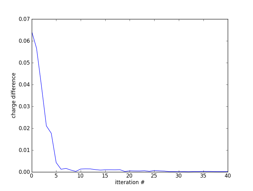
We can see that one dmft iteration takes approximately 2 minutes, while converging DFT takes 7 minutes. We therefore decided to perform 3 DMFT iterations (max_dmft_iterations=3) per global loop, so that the times used in DMFT and DFT are balanced. Once we are close to the self-consistent solution, the charge will more rapidly converge, and we might want to set max_dmft_iterations=1 and perhaps increase the number of Monte Carlo steps (M) a bit.
We can check the convergence of the charge by "grep ':CHARGE' LaVO3.dayfile" and plotting the result shows

quite rapid convergence. The impurity/local Green's function at the first few iteration is metallic, but from the third iteration on, it is nicely insulating:

and is very well converged within a dozen DMFT iterations

Notice that the speed of convergence might be somewhat different under slightly different circumstances, but the final result should be the same. The self-energy develops a pole in the gap (on the real axis). Since the pole is not exactly at the chemical potential, the imaginary part of the matsubara self-energy does not diverge at zero, but just becomes very enhanced at some finite frequency of the order of the pole energy

Another important file to check is the info.iterate, which contains information about the chemical potential, the number of electrons on the V ion, etc:

  #   #.   #           mu          Vdc            Etot     Ftot+T*Simp     Ftot+T*Simp       n_latt        n_imp      Eimp[0]     Eimp[-1] 
  0   0.   0    10.802683     8.600000   -77387.465954   -77387.477585   -77387.466952     2.090801     2.318802     0.006467    -0.032436 
  1   0.   1    10.802683     8.600000   -77387.465340   -77387.492802   -77387.466489     2.093282     2.318802     0.006467    -0.032436 
  2   0.   2    10.802683     8.600000   -77387.464174   -77387.539134   -77387.465772     2.100792     2.318802     0.006467    -0.032436 
  3   0.   3    10.802683     8.600000   -77387.467889   -77387.582991   -77387.468670     2.108055     2.318802     0.006467    -0.032436 
  4   0.   4    10.802683     8.600000   -77387.467008   -77387.459389   -77387.466007     2.093235     2.318802     0.006467    -0.032436 
  5   0.   5    10.802683     8.600000   -77387.465826   -77387.432207   -77387.465538     2.099350     2.318802     0.006467    -0.032436 
  6   0.   6    10.802683     8.600000   -77387.465089   -77387.445521   -77387.465007     2.098870     2.318802     0.006467    -0.032436 
  7   0.   7    10.802683     8.600000   -77387.465332   -77387.460681   -77387.465192     2.098445     2.318802     0.006467    -0.032436 
  8   0.   8    10.802683     8.600000   -77387.465360   -77387.462474   -77387.465236     2.098569     2.318802     0.006467    -0.032436 
  9   0.   9    10.802683     8.600000   -77387.465362   -77387.461951   -77387.465233     2.098513     2.318802     0.006467    -0.032436 
 10   1.   0    10.802683     8.600000   -77387.460012   -77387.469787   -77387.460220     2.094443     2.095318    -0.045519    -0.033396 
 11   1.   1    10.802683     8.600000   -77387.460005   -77387.472545   -77387.460267     2.094928     2.095318    -0.045519    -0.033396 
 12   1.   2    10.802683     8.600000   -77387.459992   -77387.480820   -77387.460413     2.096383     2.095318    -0.045519    -0.033396 
 13   1.   3    10.802683     8.600000   -77387.459909   -77387.496109   -77387.460596     2.099164     2.095318    -0.045519    -0.033396 
 14   1.   4    10.802683     8.600000   -77387.459849   -77387.483230   -77387.460247     2.097002     2.095318    -0.045519    -0.033396 
 15   1.   5    10.802683     8.600000   -77387.459837   -77387.482892   -77387.460233     2.096926     2.095318    -0.045519    -0.033396 
 16   1.   6    10.802683     8.600000   -77387.459826   -77387.483043   -77387.460230     2.096961     2.095318    -0.045519    -0.033396 
 17   2.   0    10.802683     8.600000   -77387.459876   -77387.469584   -77387.459850     2.093987     2.095365    -0.047880    -0.020161 
 18   2.   1    10.802683     8.600000   -77387.459888   -77387.471608   -77387.459903     2.094331     2.095365    -0.047880    -0.020161 
 19   2.   2    10.802683     8.600000   -77387.459926   -77387.477680   -77387.460062     2.095364     2.095365    -0.047880    -0.020161 
 20   2.   3    10.802683     8.600000   -77387.459982   -77387.483555   -77387.460234     2.096339     2.095365    -0.047880    -0.020161 
 21   2.   4    10.802683     8.600000   -77387.460087   -77387.481466   -77387.460288     2.095811     2.095365    -0.047880    -0.020161 
 22   2.   5    10.802683     8.600000   -77387.460124   -77387.481317   -77387.460310     2.095700     2.095365    -0.047880    -0.020161 
 23   3.   0    10.802683     8.600000   -77387.460261   -77387.469926   -77387.460626     2.095151     2.095499    -0.048408    -0.024003 
 24   3.   1    10.802683     8.600000   -77387.460262   -77387.470303   -77387.460635     2.095216     2.095499    -0.048408    -0.024003 
 25   3.   2    10.802683     8.600000   -77387.460266   -77387.471434   -77387.460663     2.095410     2.095499    -0.048408    -0.024003 
 26   3.   3    10.802683     8.600000   -77387.460275   -77387.473579   -77387.460725     2.095763     2.095499    -0.048408    -0.024003 
 27   3.   4    10.802683     8.600000   -77387.460279   -77387.472274   -77387.460704     2.095511     2.095499    -0.048408    -0.024003 
 28   4.   0    10.802683     8.600000   -77387.460351   -77387.470022   -77387.460459     2.094666     2.095620    -0.045926    -0.027269 
 29   4.   1    10.802683     8.600000   -77387.460353   -77387.470562   -77387.460473     2.094760     2.095620    -0.045926    -0.027269 
 30   4.   2    10.802683     8.600000   -77387.460356   -77387.472183   -77387.460512     2.095043     2.095620    -0.045926    -0.027269 
 31   4.   3    10.802683     8.600000   -77387.460384   -77387.475853   -77387.460635     2.095674     2.095620    -0.045926    -0.027269 
 32   4.   4    10.802683     8.600000   -77387.460392   -77387.473435   -77387.460594     2.095216     2.095620    -0.045926    -0.027269 
 33   4.   5    10.802683     8.600000   -77387.460402   -77387.473051   -77387.460590     2.095111     2.095620    -0.045926    -0.027269 
 34   4.   6    10.802683     8.600000   -77387.460408   -77387.473298   -77387.460600     2.095147     2.095620    -0.045926    -0.027269 
 35   5.   0    10.802683     8.600000   -77387.460663   -77387.470346   -77387.460609     2.094289     2.095708    -0.049409    -0.033571 
 36   5.   1    10.802683     8.600000   -77387.460667   -77387.470932   -77387.460625     2.094389     2.095708    -0.049409    -0.033571 
 37   5.   2    10.802683     8.600000   -77387.460678   -77387.472692   -77387.460672     2.094688     2.095708    -0.049409    -0.033571 
 38   5.   3    10.802683     8.600000   -77387.460706   -77387.475868   -77387.460765     2.095216     2.095708    -0.049409    -0.033571 
 39   5.   4    10.802683     8.600000   -77387.460726   -77387.473877   -77387.460746     2.094822     2.095708    -0.049409    -0.033571 
 40   6.   0    10.802683     8.600000   -77387.460778   -77387.470485   -77387.461255     2.095445     2.095610    -0.048972    -0.036624 
 41   6.   1    10.802683     8.600000   -77387.460769   -77387.470152   -77387.461240     2.095391     2.095610    -0.048972    -0.036624 
 42   6.   2    10.802683     8.600000   -77387.460745   -77387.469155   -77387.461198     2.095231     2.095610    -0.048972    -0.036624 
 43   6.   3    10.802683     8.600000   -77387.460605   -77387.466208   -77387.461009     2.094845     2.095610    -0.048972    -0.036624 
 44   6.   4    10.802683     8.600000   -77387.460597   -77387.467710   -77387.461035     2.095142     2.095610    -0.048972    -0.036624 
 45   7.   0    10.802683     8.600000   -77387.460594   -77387.470275   -77387.461146     2.095728     2.095578    -0.039428    -0.040639 
 46   7.   1    10.802683     8.600000   -77387.460591   -77387.469916   -77387.461136     2.095666     2.095578    -0.039428    -0.040639 
 47   7.   2    10.802683     8.600000   -77387.460584   -77387.468840   -77387.461108     2.095482     2.095578    -0.039428    -0.040639 
 48   8.   0    10.802683     8.600000   -77387.460559   -77387.470247   -77387.461008     2.095405     2.095454    -0.039692    -0.039728 
 49   8.   1    10.802683     8.600000   -77387.460558   -77387.470382   -77387.461009     2.095429     2.095454    -0.039692    -0.039728 
 50   8.   2    10.802683     8.600000   -77387.460556   -77387.470785   -77387.461015     2.095503     2.095454    -0.039692    -0.039728 
 51   8.   3    10.802683     8.600000   -77387.460529   -77387.471589   -77387.461000     2.095678     2.095454    -0.039692    -0.039728 
 52   8.   4    10.802683     8.600000   -77387.460519   -77387.470835   -77387.460976     2.095560     2.095454    -0.039692    -0.039728 
......
132  26.   6    10.802683     8.600000   -77387.460758   -77387.471728   -77387.461001     2.095030     2.095637    -0.036717    -0.048059 
133  27.   0    10.802683     8.600000   -77387.460615   -77387.470313   -77387.461025     2.095406     2.095589    -0.038881    -0.050831 
134  27.   1    10.802683     8.600000   -77387.460613   -77387.470035   -77387.461017     2.095359     2.095589    -0.038881    -0.050831 
135  27.   2    10.802683     8.600000   -77387.460607   -77387.469200   -77387.460995     2.095217     2.095589    -0.038881    -0.050831

This log file shows 8 DFT+DMFT cycles, and at each cycle there are 4-10 DFT steps (column 3). The chemical potential (column 4) is fixed, as well as the double-counting (this is because we choose DCs='nominal' in params.dat file. We could choose DCs='exactd', which would give similar results, but would take more time to converge). The next two columns shows total energy and free energy. Finally columns 9 and 10 show the impurity and lattice occupancy, which should match once the loop is converged. The last two columns show the first and the last impurity level.

At this point, we can proceed to the next step.

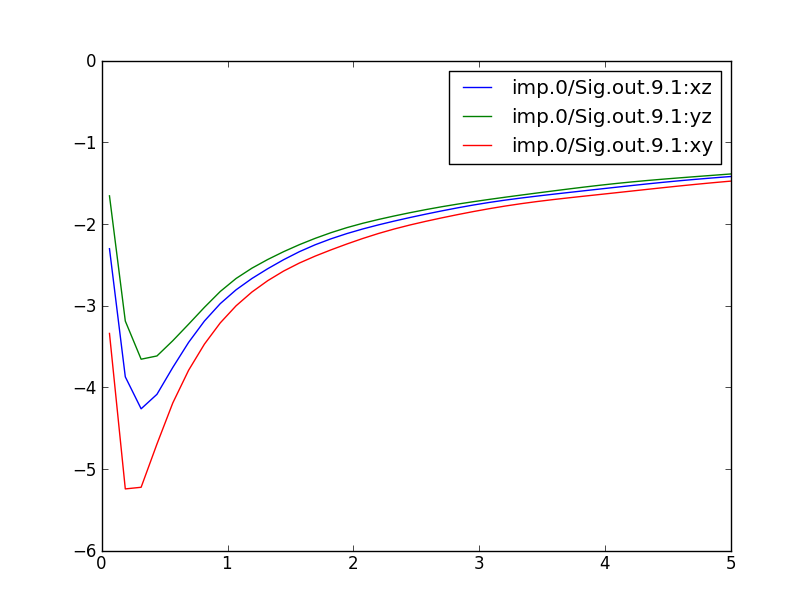
Once the calculation is done on the imaginary axis, we need to do analytical continuation to obtain the self energy on the real axis. For this,we first take average of the sig.inp files from the last few steps (in order to reduce the noise) by

saverage.py sig.inp.30.?

This script creates the averaged file sig.inpx. Next, create a new directory, and copy the averaged self energy sig.inpx to this working directory. Also copy the maxent_params.dat file, which contains the parameters for the analytical continuation process. Then run

maxent_run.py sig.inpx

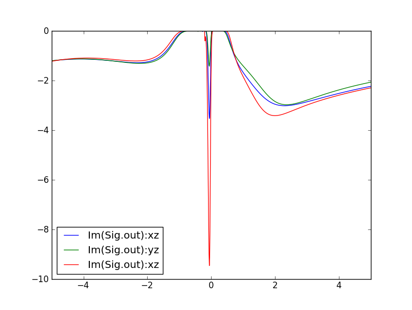
which uses the maximum entropy method to do analytical continuation. This creates the self energy Sig.out on the real axis. The imaginary part of self-energy should be similar to this plot:

The precise form will of course differ, as small difference in input data can give quite different analytically continued self-energy. But the spectra should be more similar. Notice the appearance of pole in the gap on the real axis. This proves the Mott nature of the gap.

A few clarifications are in order. Such self-energy with a pole-like structure can not be analytically continued with maax-entropy method. The high-quality of this self-energy on real-axis is due to a trick that we use: We cobstruct a new auxiliary object, which has the following form Gt(i*w)=1/(i*w-Sigma(i*w)+Sigma(infty)). This quantity is analytic (as all other quantities like Sigma and G) and has a gap when self-energy diverges. Similarly to the DMFT green's function, it is quite well-behaved on the real axis, and can be easily continued to the real axis. Once we have Im(Gt(w)) on the real axis, we perform the Kramars-Kronig transformation to obtain complex Gt(w). From that, we get self-energy as Sigma(w)=w-1/Gt(w)+Sigma(infty).

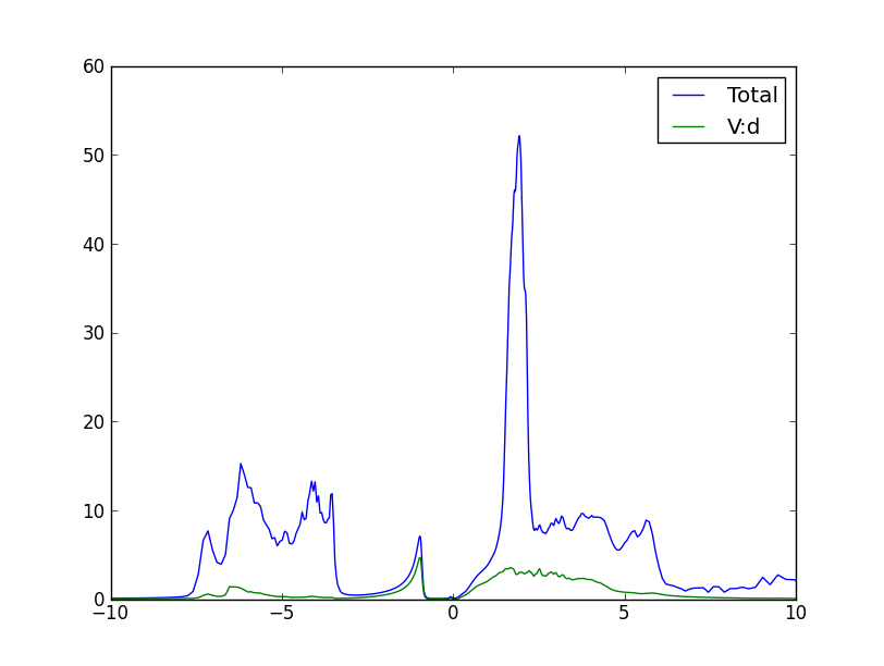
Now we need to make one last dmft1 calculation in order to obtain the Green's function and DOS on the real axis. Create a new directory, and use "dmft_copy.py <dmft_results>" to copy necessary files from the output of the DMFT run to the new directory. Also copy the analytically continued self energy Sig.out to sig.inp to this new directory. Since we need to run the code on the real axis, we need to change the .indmfl file. The first number on the second line of .indmfl file determines whether the code is run on the real axis (0) or the imaginary axis (1). Change it to 0. Then, run

x lapw0 -f  LaVO3
x_dmft.py lapw1
x_dmft.py dmft1

respectively.

Once the run is done, we now have the densities of states on the real axis. Both the partial (V-d) and the total DOS is stored in the 'LaVO3.cdos' file:

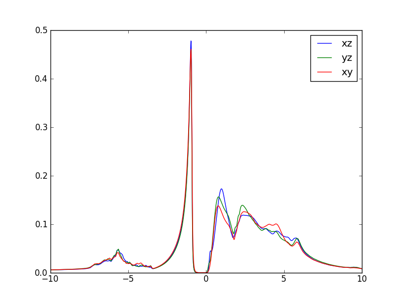
We can also take a look at the imaginary part of the green's function. Recall that the imaginary part of the green's function, divided by -pi, gives the DOS. So, plotting the even-numbered columns in the .gc1, we can get the DOS of individual d orbitals. It looks like this:

Another quantity of physical interest is the momentum resolved spectral function, which is an equivalent of spaghetti plot in DFT. First, we need to select a path in momentum space and store it into LaVO3.klist_band. One simple way is to open "xcrysden" and select option "File/Open-WIEN2k/Select-k-path". Alternatively, one could select from one of the Wien2k prepared templates. Next, we run Wien2k on the selected path, i.e.,

x lapw0 -f LaVO3
x_dmft.py lapw1 --band

We then edit LaVO3.indmfl file, to make sure that the matsubara flag is set to 0, and in the same line, one could can the number of frequency points (4-th number), and frequency range (number 5 and 6) for the plot. In this line we will set:

0 0.025 0.025 200 -3.000000 3.000000  # matsubara, broadening-corr, broadening-noncorr, nomega, omega_min, omega_max (in eV)

which selects 200 points in the range of -3eV and 3eV. Finally, we run dmftp step to compute the DMFT eigenvalues on this mesh:

x_dmft.py dmftp

Next, we need to make sure that "EF.dat" exist. Normally, it should be created during the self-consistent run, except if the chemical potential is fixed (as it was done here). If file EF.dat does not exist, we can just find the chemical potential in info.iterate and write it into EF.dat.

echo 10.802683 > EF.dat

Note that a single real number is expected in this file. Alternatively, we could also find the chemical potential by "grep ':FER' LaVO3.scf2" and convert it from Ry to eV.

Next we execute

wakplot.py

to obtain the plot. If the plot appears too dim, one can increase brightness by selecting the upper cutoff for the colormap. One can give a real number (intensity) as an argument to

wakplot.py 0.2

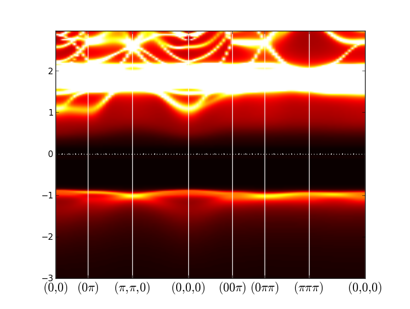
By default, the real number is 0.2. To increase the intensity, reduce this number. In order to see clearly the incoherent spectral weight of the lower Hubbard band, one might need to reduce the intensity to 0.03. Here is how the plot should look like:

.
Note that the very bright set of bands around 2eV are La-f states.

Tutorial 4: LaVO3

Obtaining transformation by findRot.py

Obtaining transformation by a series of steps

The rest of initialization

Tutorial 4: LaVO₃