Home What is? Install Overview CTQMC MnO FeSe SrVO3 LaVO3 Cerium Sr2IrO4 Ta2NiSe5 phonon

Tutorial 3: SrVO₃

Tutorial 3.a. : Preparing the job

Next, we will discuss the correlated metal SrVO₃. This compound is a perovskite, with 5 atoms in the unit cell. The V⁴⁺ ion formally has one electron in its d-shell. We will treat dynamically this t2g electron using DMFT.

This time we will start from the standard crystallographic format SrVO3.cif file, which was generated by findsym tool. A new script in 2024 version is available to handle cif files, namely cif2struct.py [Note that this tool should work for monoclinic structures for which w2k cif2struct is buggy, it should also work with output from VESTA or output from findsym programs]. We can run

cif2struct.py SrVO3.cif

to obtain SrVO3.struct file.
We can also add options -w to print case.klist_band file for plotting spectral function of DMFT, or spaghetti of wien2k:

cif2struct.py -w -N 300 SrVO3.cif

You can look at cif2struct.log file, which contains a lot of information on conversion. The help is also available for the script "--help", which should allow for more options.

Next we run Wien2k initialization using init_lapw and default options. In version 14, one types the following

  
Enter reduction in %:   0
Use old or new scheme (o/N) : N
Do you want to accept these radii; .... (a/d/r) : a
specify nn-bondlength factor: 2
Ctrl-X-C
continue with sgroup : c
Ctrl-X-C
continue with symmetry : c
Ctrl-X-C
continue with lstart : c
specify switches for instgen_lapw (or press ENTER): ENTER
SELECT XCPOT: 5
SELECT ENERGY : -6
Ctrl-X-C
continue with kgen : c
Ctrl-X-C
Ctrl-X-C
NUMBER OF K-POINTS : 500
Shift of k-mesh (0=no, 1=shift) : 1
Ctrl-X-C
c
Ctrl-X-C
n

Here Ctrl-X-C stands for breaking out of your editor.

We chose to work with LDA functional, and use a shifted k-point grid of 500 points (in the whole Brillouin zone), and we neglected spin-orbit coupling.

Next, run the DFT calculation by

run_lapw

To calculate the local Green's function we will increase the number of k-points to 2000 by

x kgen

and specify 2000 k-points with shifted k-mesh. Next, we rerun wien2k on this k-mesh by

run_lapw

Next we initialize the DMFT files by the python script init_dmft.py, and choose the following options

Specify correlated atoms (ex: 1-4,7,8):  1

Do you want to continue; or edit again? (c/e): c

For each atom, specify correlated orbital(s) (ex: d,f):
  1 V: d

Do you want to continue; or edit again? (c/e): c

Specify qsplit for each correlated orbital (default = 0):
  1  V-1 d: 3

Do you want to continue; or edit again? (c/e): c

Specify projector type (default = 2): 5

Do you want to continue; or edit again? (c/e): c

Do you want to group any of these orbitals into cluster-DMFT problems? (y/n): n

Enter the correlated problems forming each unique correlated
problem, separated by spaces (ex: 1,3 2,4 5-8): 1

Do you want to continue; or edit again? (c/e): c

Range (in eV) of hybridization taken into account in impurity
problems; default -10.0, 10.0: 

Perform calculation on real; or imaginary axis? (r/i): i

Ctrl-X-C

Is this a spin-orbit run? (y/n): n

Ctrl-X-C

Most of the options were explained in the previous tutorials. Here we will discuss only those options which differ from preceding examples.

At the beginning, the code shows all atoms in the unit cell:
There are 5 atoms in the unit cell: 1 V 2 Sr 3 O 4 O 5 O Specify correlated atoms (ex: 1-4,7,8): 1
and asks which one should be treated dynamically. We choose only the V atom to be treated dynamically by the DMFT.
The code next asks which orbital quantum numbers should be treated dynamically:
For each atom, specify correlated orbital(s) (ex: d,f): 1 V: d
The partially filled d shell of the V ion is to be treated in DMFT.

Next we should specify what type of local symmetry we have on the given atom, and if we possibly want to correlated only a sub-shell

Specify qsplit for each correlated orbital (default = 0): Qsplit Description ------ ------------------------------------------------------------ 0 average GF, non-correlated 1 |j,mj> basis, no symmetry, except time reversal (-jz=jz) -1 |j,mj> basis, no symmetry, not even time reversal (-jz=jz) 2 real harmonics basis, no symmetry, except spin (up=dn) -2 real harmonics basis, no symmetry, not even spin (up=dn) 3 t2g orbitals -3 eg orbitals 4 |j,mj>, only l-1/2 and l+1/2 5 axial symmetry in real harmonics 6 hexagonal symmetry in real harmonics 7 cubic symmetry in real harmonics 8 axial symmetry in real harmonics, up different than down 9 hexagonal symmetry in real harmonics, up different than down 10 cubic symmetry in real harmonics, up different then down 11 |j,mj> basis, non-zero off diagonal elements 12 real harmonics, non-zero off diagonal elements 13 J_eff=1/2 basis for 5d ions, non-magnetic with symmetry 14 J_eff=1/2 basis for 5d ions, no symmetry ------ ------------------------------------------------------------ 1 V-1 d: 3

In SrVO3, we ignored the spin-orbit coupling, and the crystal symmetry is cubic, hence hybridization is exactly diagonal in the cubic harmonics basis. We thus want to use this basis. Moreover, t_2g states are quite nicely separated from e_g states, hence we choose to correlated the t_2g states only.
It is possible to treat by DMFT the entire d-shell (option 7 or 2), and one can check that the results are very similar to the current choice (taking option 3), provided that the Coulomb U is slightly increased when the entire d shell is treated dynamically.

By choosing to correlated the t2g shell only, we will save quite a bit of computational time, as well as have the calculation converge easier.

Note that this does not mean that the e_g states are not taken into account; they are still fully taken into account at the DFT level, but just not at the DMFT level. In particular, the hybridization between the oxygen ions and the e_g states are included in DFT.

The init_dmft.py script just created two input files, SrVO3.indmfl and SrVO3.indmfi, which are needed later. The header of the SrVO3.indmfl file should look like:

12 31 1 5                             # hybridization band index nemin and nemax, renormalize for interstitials, projection type
1 0.025 0.025 200 -3.000000 1.000000  # matsubara, broadening-corr, broadening-noncorr, nomega, omega_min, omega_max (in eV)
1                                     # number of correlated atoms
1     1   0                           # iatom, nL, locrot
  2   3   1                           # L, qsplit, cix

The first line specifies the hybridization window (from band 12 to band 31) and type of the projector (projector 5).
The second line contains a switch for the real-axis/imaginary-axis calculation. We set matsubara to 1. The second line also contains information on small lorentzian broadening in k-point summation.
The third line specifies the number of correlated atoms
The forth line specifies which atom (from SrVO3.struct) is correlated (Note that each atom in the structure file counts, even when several atoms in structure files are equivalent). The forth line also specifies how many orbital indeces (different L's) we will use for projection, and calculation of local green's function and partial dos. The last index "locrot" is used for rotation of local axis, and is not needed here (set to 0).
The fifth line specifies orbital momentum "l=2", "qsplit=3" which we choose during initialization. Each correlated orbital-set gets a unique index during initialization. This correlated set was given index "cix=1". For each correlated set, a more detailed specification is needed, which is given in the remaining of "case.indmfl" file.

The specification of correlated set is given in the second part of case.indmfl:

#================ # Siginds and crystal-field transformations for correlated orbitals ================
1     5   3       # Number of independent kcix blocks, max dimension, max num-independent-components
1     5   3       # cix-num, dimension, num-independent-components
#---------------- # Independent components are --------------
'xz' 'yz' 'xy'
#---------------- # Sigind follows --------------------------
1 0 0 0 0
0 2 0 0 0
0 0 3 0 0
0 0 0 0 0
0 0 0 0 0
#---------------- # Transformation matrix follows -----------
 0.00000000 0.00000000   0.70710679 0.00000000   0.00000000 0.00000000  -0.70710679 0.00000000   0.00000000 0.00000000
 0.00000000 0.00000000   0.00000000 0.70710679   0.00000000 0.00000000   0.00000000 0.70710679   0.00000000 0.00000000 
-0.70710679 0.00000000   0.00000000 0.00000000   0.00000000 0.00000000   0.00000000 0.00000000   0.70710679 0.00000000
 0.00000000 0.00000000   0.00000000 0.00000000   1.00000000 0.00000000   0.00000000 0.00000000   0.00000000 0.00000000
 0.70710679 0.00000000   0.00000000 0.00000000   0.00000000 0.00000000   0.00000000 0.00000000   0.70710679 0.00000000

The first line specifies the number of all correlated blocks, the dimension of the largest correlated block, and number of orbital components which differ. Note that we allowed the three t_2g's to differ, although due to cubic symmetry they should turn out to be equal. [ If we want to improve statistics of ctqmc a bit, we could change this file, and give all three orbitals the same index 1 in Sigind. We would also need to change num-independent-components and max num-independent-components to 1. (see below)]

The second line specifies the dimension of the first correlated block (here "d" has dimension 5), and the three t2g components are treated as independent.

Note that the orbitals, which have index "0" in the Sigind block are treated statically. It is desirable to rearrange the orbitals in such a way that the correlated orbitals are listed first, followed by those, which are not correlated. This is already done here, but if it was not, we would permute the index table Sigind simultaneously with the rows of Transformation matrix. Namely, each row in the transformation matrix corresponds to a correlated orbital, for example row 4 is the z^2 orbital (equivalent to Y_{2,0}). As the forth diagonal element in Sigind is set to zero, this orbital is not correlated. The first three rows in Transformation matrix are familiar xz,yz,xy orbitals, and are correlated in Sigind block. Note also that the phase of each correlated orbital can be arbitrarily chosen, and the physical observables should not depend on that choice. To keep compatibility with Wien2k choice, we sometimes use i*xy, rather than xy orbital.

As explained above, we could alternatively use the symmetry and treat all three t_2g states as degenerate. In this case the indmfl would take the form

#================ # Siginds and crystal-field transformations for correlated orbitals ================
1     5   1       # Number of independent kcix blocks, max dimension, max num-independent-components
1     5   1       # cix-num, dimension, num-independent-components
#---------------- # Independent components are --------------
't2gs' 
#---------------- # Sigind follows --------------------------
1 0 0 0 0
0 1 0 0 0
0 0 1 0 0
0 0 0 0 0
0 0 0 0 0
#---------------- # Transformation matrix follows -----------
....

Next create a new folder, and when in that folder, use the command

dmft_copy.py <lda_results_directory>

where <lda_results_directory> is the directory where the output of the DFT calculation with DMFT initialization is. This command copies the necessary files to start a DMFT calculation. These include the .struct file as well as the various Wien2K input files such as .inm, .in1, etc. The charge density file, .clmsum, is also copied. This is all we need from the initial Wien2K run, and now we proceed to create the rest of the files, needed by the DMFT calculation.

Copy the params.dat file. This file contains information about the impurity solver and additional parameteres, which appear in DFT+EDMFT. Its content is:

solver         =  'CTQMC'   # impurity solver
DCs            =  'exact'   # exact double-counting with dielectric constant approx.

max_dmft_iterations = 1     # number of iteration of the dmft-loop only
max_lda_iterations  = 100   # number of iteration of the LDA-loop only
finish         =  50        # number of iterations of full charge loop (1 = no charge self-consistency)

ntail          =  300       # on imaginary axis, number of points in the tail of the logarithmic mesh

cc             =  5e-5      # the charge density precision to stop the LDA+DMFT run
ec             =  5e-5      # the energy precision to stop the LDA+DMFT run
recomputeEF    =  1         # Recompute EF in dmft2 step. If recomputeEF = 0, it fixed the chemical potential. Good for insulators
#mix_delta = 0.5            # If instability occurs, we should start mixing hybridization

# Impurity problem number 0
iparams0={"exe"                : ["ctqmc"              , "# Name of the executable"],
          "U"                  : [8.0                  , "# Coulomb repulsion (F0)"],
          "J"                  : [0.8                  , "# Coulomb repulsion (F0)"],
          "CoulombF"           : ["'Ising'"            , "# Form of Coulomb repulsion. 'Full' allows rotational invariant form of C.I."],
          "beta"               : [50                   , "# Inverse temperature T=116K"],
          "svd_lmax"           : [25                   , "# We will use SVD basis to expand G, with this cutoff"],
          "M"                  : [5e6                 , "# Total number of Monte Carlo steps"],
          "mode"               : ["SH"                 , "# We will use self-energy sampling, and Hubbard I tail"],
          "nom"                : [200                  , "# Number of Matsubara frequency points sampled"],
          "tsample"            : [200                  , "# How often to record measurements"],
          "GlobalFlip"         : [1000000              , "# How often to try a global flip"],
          "warmup"             : [3e5                  , "# Warmup number of QMC steps"],
          "nf0"                : [1.0                  , "# Nominal occupancy nd for double-counting"],
          }

All the variables were already explained in preceding tutorials. For completness, let us just emphasize here that we use the exact double-counting (see PRL 115, 196403), in which the Coulomb repulsion in real space is screened by the combination of yukawa and dielectric function.

We also need a blank self-energy file (sig.inp), which we will generate by

szero.py

Now we can run the DFT+EDMFTF calculation. Do not forget to create files for mpi execution, which should be called mpi_prefix.dat and mpi_prefix.dat2. A command similar to the following, should create them:

echo "mpiexec  -port $port -np $NSLOTS -machinefile $TMPDIR/machines" > mpi_prefix.dat 
$WIEN_DMFT_ROOT/createDMFprefix.py $JOBNAME.klist mpi_prefix.dat > mpi_prefix.dat2

The DMFT script should be run by

$WIEN_DMFT_ROOT/run_dmft.py > nohup.dat 2>&1

Before submitting the job, also make sure that the following environmental variable are set

export WIENROOT=<wien-instalation-dir>
export WIEN_DMFT_ROOT=<dir-containing-dmft-executables>
export SCRATCH="."
export PYTHONPATH=$PYTHONPATH:$WIEN_DMFT_ROOT

It is advisable to add executables to path,

export PATH=$PATH:$WIENROOT:$WIEN_DMFT_ROOT

or, one should call executables with the long pathnames:

Tutorial 3.b. : Running the job

While the code is running, there are multiple files that you can check to see how it is going. One is the ':log' file, which serves exactly the same purpose as in Wien2K. It lists the individual modules that are being run and their order:

Sat Mar 25 20:27:19 EDT 2017> (x) -f SrVO3 lapw0
Sat Mar 25 20:27:37 EDT 2017>     lapw1
Sat Mar 25 20:27:39 EDT 2017>     dmft1
Sat Mar 25 20:27:42 EDT 2017>     impurity
Sat Mar 25 20:30:45 EDT 2017>     dmft2
Sat Mar 25 20:30:48 EDT 2017> (x) -f SrVO3 lcore
Sat Mar 25 20:30:49 EDT 2017> (x) -f SrVO3 mixer
Sat Mar 25 20:30:50 EDT 2017> (x) -f SrVO3 lapw0
Sat Mar 25 20:30:53 EDT 2017>     lapw1
Sat Mar 25 20:30:55 EDT 2017>     dmft2
Sat Mar 25 20:30:58 EDT 2017> (x) -f SrVO3 lcore
Sat Mar 25 20:30:59 EDT 2017> (x) -f SrVO3 mixer
Sat Mar 25 20:31:00 EDT 2017> (x) -f SrVO3 lapw0
Sat Mar 25 20:31:03 EDT 2017>     lapw1
Sat Mar 25 20:31:05 EDT 2017>     dmft2
Sat Mar 25 20:31:08 EDT 2017> (x) -f SrVO3 lcore
Sat Mar 25 20:31:09 EDT 2017> (x) -f SrVO3 mixer
Sat Mar 25 20:31:10 EDT 2017> (x) -f SrVO3 lapw0
Sat Mar 25 20:31:12 EDT 2017>     lapw1
Sat Mar 25 20:31:15 EDT 2017>     dmft2
Sat Mar 25 20:31:19 EDT 2017> (x) -f SrVO3 lcore
Sat Mar 25 20:31:20 EDT 2017> (x) -f SrVO3 mixer
Sat Mar 25 20:31:21 EDT 2017> (x) -f SrVO3 lapw0
Sat Mar 25 20:31:23 EDT 2017>     lapw1
Sat Mar 25 20:31:25 EDT 2017>     dmft2
Sat Mar 25 20:31:29 EDT 2017> (x) -f SrVO3 lcore
Sat Mar 25 20:31:30 EDT 2017> (x) -f SrVO3 mixer
Sat Mar 25 20:31:31 EDT 2017> (x) -f SrVO3 lapw0
Sat Mar 25 20:31:33 EDT 2017>     lapw1
Sat Mar 25 20:31:35 EDT 2017>     dmft2
Sat Mar 25 20:31:38 EDT 2017> (x) -f SrVO3 lcore
Sat Mar 25 20:31:39 EDT 2017> (x) -f SrVO3 mixer
Sat Mar 25 20:31:40 EDT 2017> (x) -f SrVO3 lapw0
Sat Mar 25 20:31:43 EDT 2017>     lapw1
Sat Mar 25 20:31:45 EDT 2017>     dmft2
Sat Mar 25 20:31:49 EDT 2017> (x) -f SrVO3 lcore
Sat Mar 25 20:31:49 EDT 2017> (x) -f SrVO3 mixer
Sat Mar 25 20:31:51 EDT 2017> (x) -f SrVO3 lapw0
.....
Sat Mar 25 20:32:50 EDT 2017> (x) -f SrVO3 lapw0
Sat Mar 25 20:32:53 EDT 2017>     lapw1
Sat Mar 25 20:32:55 EDT 2017>     dmft1
Sat Mar 25 20:32:57 EDT 2017>     impurity
Sat Mar 25 20:34:39 EDT 2017>     dmft2
Sat Mar 25 20:34:43 EDT 2017> (x) -f SrVO3 lcore
Sat Mar 25 20:34:43 EDT 2017> (x) -f SrVO3 mixer
Sat Mar 25 20:34:45 EDT 2017> (x) -f SrVO3 lapw0

The code starts by running the lapw0 and lapw1 modules of Wien2K to calculate the vector files, etc; but then, dmft1 is called to calculate hybridization function. The impurity solver is called between dmft1 and dmft2, and then charge self-consistent dft loop is repeated many times (dmft2, core, mixer, lapw0, lapw1). We choose this option, because the DFT part is here very fast (much faster than the impurity solver), so many DFT steps (up to max_lda_iterations=100) are performed in combination with a single dmft step (max_dmft_iterations=1). Once the charge loop is done (either charge and energy are converged [cc \& ec], or we exceeded max_lda_iterations), the dmft1 step is called again, followed by the impurity solver.

Whether the charge density got well converged can be checked by grep'ing ':CHARGE' in the .dayfile:

:CHARGE convergence:  1.0
:CHARGE convergence:  0.0835935
:CHARGE convergence:  0.0439781
:CHARGE convergence:  0.0657028
:CHARGE convergence:  0.0459584
:CHARGE convergence:  0.0432044
:CHARGE convergence:  0.0043898
:CHARGE convergence:  0.0063747
:CHARGE convergence:  0.0034868
:CHARGE convergence:  0.0016732
:CHARGE convergence:  0.0003244
:CHARGE convergence:  5.52e-05
:CHARGE convergence:  1.36e-05
:CHARGE convergence:  0.0052109
:CHARGE convergence:  0.0045152
:CHARGE convergence:  0.0025189
:CHARGE convergence:  0.0027001
:CHARGE convergence:  0.0007694
:CHARGE convergence:  0.0004947
:CHARGE convergence:  0.0001302
:CHARGE convergence:  3.72e-05

Note that while the charge converges quite well within the DFT loop, after the dmft1 step it is again non-converged, since the self energy was updated. Towards the end of the run (after about 30 cycles), the self energy is also well converged and so the jump in the charge after each dmft1 step, is much less significant:

:CHARGE convergence:  6.4e-05
:CHARGE convergence:  5.16e-05
:CHARGE convergence:  7.82e-05
:CHARGE convergence:  3.24e-05
:CHARGE convergence:  2.87e-05
:CHARGE convergence:  3.05e-05
:CHARGE convergence:  2.62e-05
:CHARGE convergence:  4.31e-05
:CHARGE convergence:  3.77e-05
:CHARGE convergence:  5.45e-05
:CHARGE convergence:  4.65e-05
:CHARGE convergence:  5.75e-05
:CHARGE convergence:  4.95e-05
:CHARGE convergence:  5.02e-05
:CHARGE convergence:  4.25e-05
:CHARGE convergence:  9.4e-06
:CHARGE convergence:  8.2e-06

Still, due to Monte Carlo noise, the charge can not converge to arbitrary high accuracy at finite Monte Carlo precision. Nonetheless, we can typically achieve precision below 1e-5, which is more accurate than usually used in DFT-LAPW calculations.

Another important file to check is the info.iterate, which contains information about the chemical potential, the number of electrons on the V ion, etc:

  #   #.   #           mu          Vdc            Etot     Ftot+T*Simp     Ftot+T*Simp       n_latt        n_imp      Eimp[0]     Eimp[-1] 
  0   0.   0     8.770334     3.881170    -8696.600092    -8696.627108    -8696.589740     1.390867     1.035714    -0.042696    -0.042696 
  1   0.   1     8.721143     3.881170    -8696.599194    -8696.671599    -8696.589452     1.403287     1.035714    -0.042696    -0.042696 
  2   0.   2     8.573921     3.881170    -8696.598217    -8696.803391    -8696.590010     1.441857     1.035714    -0.042696    -0.042696 
  3   0.   3     8.202136     3.881170    -8696.605608    -8697.122541    -8696.601390     1.551790     1.035714    -0.042696    -0.042696 
  4   0.   4     8.460228     3.881170    -8696.598488    -8696.841630    -8696.590804     1.460942     1.035714    -0.042696    -0.042696 
  5   0.   5     8.147676     3.881170    -8696.605366    -8697.102050    -8696.601312     1.556594     1.035714    -0.042696    -0.042696 
  6   0.   6     8.373934     3.881170    -8696.600005    -8696.929838    -8696.593972     1.498405     1.035714    -0.042696    -0.042696 
  7   0.   7     8.317077     3.881170    -8696.600855    -8696.972107    -8696.595356     1.511839     1.035714    -0.042696    -0.042696 
  8   0.   8     8.325935     3.881170    -8696.600578    -8696.965302    -8696.594961     1.508504     1.035714    -0.042696    -0.042696 
  9   0.   9     8.333896     3.881170    -8696.600401    -8696.958379    -8696.594737     1.506428     1.035714    -0.042696    -0.042696 
 10   0.  10     8.339930     3.881170    -8696.600365    -8696.953237    -8696.594558     1.504693     1.035714    -0.042696    -0.042696 
 11   0.  11     8.341431     3.881170    -8696.600332    -8696.952012    -8696.594515     1.504284     1.035714    -0.042696    -0.042696 
 12   0.  12     8.341274     3.881170    -8696.600336    -8696.952123    -8696.594520     1.504328     1.035714    -0.042696    -0.042696 
 13   1.   0     8.309814     4.371950    -8696.593956    -8696.597300    -8696.590861     1.480979     1.114940    -0.789484    -0.789484 
 14   1.   1     8.307926     4.371950    -8696.594006    -8696.598954    -8696.590931     1.481605     1.114940    -0.789484    -0.789484 
 15   1.   2     8.302265     4.371950    -8696.594162    -8696.603913    -8696.591144     1.483484     1.114940    -0.789484    -0.789484 
 16   1.   3     8.289969     4.371950    -8696.594473    -8696.614043    -8696.591648     1.487772     1.114940    -0.789484    -0.789484 
 17   1.   4     8.298014     4.371950    -8696.594307    -8696.601976    -8696.591415     1.485486     1.114940    -0.789484    -0.789484 
 18   1.   5     8.295568     4.371950    -8696.594356    -8696.604601    -8696.591467     1.486003     1.114940    -0.789484    -0.789484 
 19   1.   6     8.294026     4.371950    -8696.594367    -8696.605882    -8696.591468     1.486078     1.114940    -0.789484    -0.789484 
 20   1.   7     8.294637     4.371950    -8696.594359    -8696.605625    -8696.591463     1.486020     1.114940    -0.789484    -0.789484 
 21   2.   0     8.320967     4.713672    -8696.589028    -8696.596377    -8696.586800     1.475189     1.169843    -0.763354    -0.763353 
......
195  29.   0     8.480065     6.490811    -8696.565894    -8696.573610    -8696.565344     1.449904     1.445104    -1.067816    -1.067892 
196  29.   1     8.480403     6.490811    -8696.565884    -8696.573243    -8696.565331     1.449812     1.445104    -1.067816    -1.067892 
197  29.   2     8.481417     6.490811    -8696.565852    -8696.572142    -8696.565292     1.449536     1.445104    -1.067816    -1.067892 
198  29.   3     8.487627     6.490811    -8696.565668    -8696.564739    -8696.565066     1.447849     1.445104    -1.067816    -1.067892 
199  29.   4     8.482462     6.490811    -8696.565826    -8696.569727    -8696.565259     1.449233     1.445104    -1.067816    -1.067892 
200  29.   5     8.482355     6.490811    -8696.565827    -8696.569881    -8696.565260     1.449244     1.445104    -1.067816    -1.067892 
201  29.   6     8.482271     6.490811    -8696.565825    -8696.570101    -8696.565258     1.449240     1.445104    -1.067816    -1.067892 
202  30.   0     8.487685     6.495397    -8696.568237    -8696.576298    -8696.566507     1.446473     1.446400    -1.065371    -1.065310 
203  30.   1     8.487229     6.495397    -8696.568251    -8696.576779    -8696.566524     1.446595     1.446400    -1.065371    -1.065310 
204  30.   2     8.485860     6.495397    -8696.568292    -8696.578220    -8696.566575     1.446962     1.446400    -1.065371    -1.065310 
205  30.   3     8.477397     6.495397    -8696.568550    -8696.587772    -8696.566884     1.449201     1.446400    -1.065371    -1.065310 
206  30.   4     8.484230     6.495397    -8696.568333    -8696.581241    -8696.566624     1.447393     1.446400    -1.065371    -1.065310 
207  30.   5     8.484380     6.495397    -8696.568332    -8696.581067    -8696.566624     1.447383     1.446400    -1.065371    -1.065310 
208  30.   6     8.484556     6.495397    -8696.568334    -8696.580786    -8696.566626     1.447377     1.446400    -1.065371    -1.065310 
209  31.   0     8.483446     6.518435    -8696.565292    -8696.572554    -8696.564673     1.449912     1.448534    -1.072144    -1.072250

The second column counts the number of DMFT steps (impurity solver), the third counts charge-dft steps at each DMFT steps, next columns shows the chemical potential, the double-counting potential, the total energy, the free energy, followed by another free energy (the latter is numerically more stable, and should be used), occupation of the atom in the solid, and the impurity occupation, and the impurity levels.

Since we are using the exact double-counting, the convergence of the impurity occupations and Vdc is rather slow (nominal double-counting would converge way faster), nevertheless, after 30 dmft iterations we see that the impurity occupation is well converged, and the material is very mixed-valent (to 1.45). This mixed-valency is the reason for SrVO3 metallicity for which even very large U can not open the gap.

The comparison on n_latt (column 9) and n_imp (column 10) is a very non-trivial check of numerics precision and convergence, as the equivalence between the local and the impurity Green's function is not imposed, but is achieved only once the self-consistency is reached. If you'd like to get more information about the details of the run, you can also monitor the files SrVO3.scf, SrVO3.outputdmf1, SrVO3.outputdmf2, dmft_info, dmft1_info.out, dmft2_info.out, imp.0/ctqmc.log, imp.0/nohup_imp.out.xxx, and many others.

Notice that most of the parameters in "params.dat" file can be changed during the run, and their value will be updated in the next start of the global loop. For example, one can change the number of charge steps ("max_lda_iterations") or dmft steps ("max_dmft_iterations") or number of Monte Carlo steps ("M") during the run to get convergence faster. It does take some experience to choose efficient set of parameters.

Sometimes a double-period appears, and the self-energy is jumping between two different values from iteration to iteration. Or the self-energy starts to jump from iteration to iteration once it was almost converged. In this case, we should mix hybridization function and the impurity levels. This is achieved by specifying

mix_delta = 0.5

In the next iteration, we will take mix_delta of the new value, and (1-mix_delta) of the old value. Note that since DMFT loop is very stable, we typically just take the new calculated quantities at each iteration, and we do not mix. Also note that if mix_delta is not successful in achieving convergence, one can also specify mix_sigma.

As mentioned above, the fastest way to check convergence is to plot the impurity and the lattice occupancy in column 9 and 10 of info.iterate

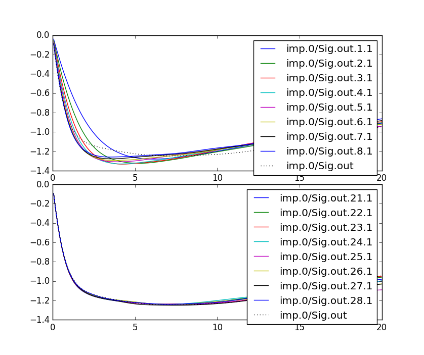
Another way to check the convergence is to plot the self-energy. The impurity self energy is stored in the 'imp.0/Sig.out.*.*' file in the. In our case, this file has seven columns: The first column is the energy, and there is a pair of columns (real and imaginary) for each orbital. Plotting the imaginary part of first few iterations, we get:

Note that "imp.0/Sig.out" file is the last self-energy after over 50 dmft iterations, hence it is well converged. We notice that while iterations 7-8 do not change much, the self-energy is not completely converged, as occupancy is still changing and the double-counting is still not converged (note that nominal DC would converge must faster). Only after 20 or so dmft iterations the self-energy is basically equal to the converged value. At that time, the difference between the impurity and lattice occupancy is of the order 1e-2, i.e., over one order of magnitude smaller than at the beginning. Note however, that the low energy value of the self-energy (mass enhancement) is quite well converged even after only a few steps. This is because in metals, the low energy self-energy, computed by CTQMC, is very stable, which makes this solver particularly suitable for DFT+DMFT calculations.

At this point, we can proceed to the next step.

Once the calculation is done on the imaginary axis, we need to do analytical continuation to obtain the self energy on the real axis. For this,we first take average of the sig.inp files from the last few steps (in order to reduce the noise) by

 saverage.py sig.inp.5?

This script creates the file sig.inpx. Next, create a new directory, and copy the averaged self energy sig.inpx into this directory. Also copy the maxent_params.dat file:

params={'statistics': 'fermi', # fermi/bose
        'Ntau'      : 400,     # Number of time points
        'L'         : 20.0,    # cutoff frequency on real axis
        'x0'        : 0.01,   # low energy cut-off
        'bwdth'     : 0.004,    # smoothing width
        'Nw'        : 300,     # number of frequency points on real axis
        'gwidth'    : 2*15.0,  # width of gaussian
        'idg'       : 1,       # error scheme: idg=1 -> sigma=deltag ; idg=0 -> sigma=deltag*G(tau)
        'deltag'    : 0.001,   # error
        'Asteps'    : 4000,    # anealing steps
        'alpha0'    : 1000,    # starting alpha
        'min_ratio' : 0.001,    # condition to finish, what should be the ratio
        'iflat'     : 1,       # iflat=0 : constant model, iflat=1 : gaussian of width gwidth, iflat=2 : input using file model.dat
        'Nitt'      : 1000,    # maximum number of outside iterations
        'Nr'        : 0,       # number of smoothing runs
        'Nf'        : 40,      # to perform inverse Fourier, high frequency limit is computed from the last Nf points
        }

which contains the parameters for the analytical continuation process. Then run

maxent_run.py sig.inpx

which uses the maximum entropy method to do analytical continuation. This creates the self energy Sig.out on the real axis. It should be similar to this plot:

Now we need to make one last dmft1 calculation in order to obtain the Green's function and DOS on the real axis. Create a new directory, and use

dmft_copy.py <dmft_results>

to copy necessary files from the output of the DMFT run to the new directory. Also copy the analytically continued self energy Sig.out to sig.inp to this new directory. Since we need to run the code on the real axis, we need to change the .indmfl file. The matsubara flag (the first number on the second line) in .indmfl file determines whether the code is run on the real axis (0) or the imaginary axis (1). Change it to 0. Then, run

x lapw0 -f  SrVO3
x_dmft.py lapw1
x_dmft.py dmft1

respectively. For nicer plot, you might want to increase the number of k-points, using

x kgen -f SrVO3

before running lapw1 step.

Once the run is done, we now have the densities of states on the real axis. Both the partial (V-d) and the total DOS is stored in the SrVO3.cdos file:

We can also take a look at the imaginary part of the green's function. Recall that the imaginary part of the green's function, divided by -pi, gives the DOS. So, plotting the even-numbered columns in the .gc1 one, we can get the DOS of individual d orbitals. After some broadening, it looks like this:

Note how nicely the upper and lower Hubbard bands, as well as the quasiparticle peak show up. However, it is clear from the large value of the Coulomb repulsion in our calculation that the peak at -1.5eV is not standard lower Hubbard band (the lower Hubbard band is connected to broad spectrum beyond -4eV), but is rather an excitation connected to strong hybridization with oxygen. Namely, hybridization pushes the spectra away from the region of large hybdiziation (below -2eV). As the electrons try to screen the low energy local moment, they create the screening cloud, which can appear in the energy region of small charge, showing up as a excitation peak.
We correlated only the t2g states, hence the eg states are not printed in the SrVO3.gc1 file, but note that they are added in SrVO3.cdos file. To plot the eg states separately (as we have done above), we can slightly modify the SrVO3.indmfl file, and add index 4 for eg-states, i.e,

12 31 1 5                             # hybridization band index nemin and nemax, renormalize for interstitials, projection type
0 0.025 0.05 200 -3.000000 1.000000  # matsubara, broadening-corr, broadening-noncorr, nomega, omega_min, omega_max (in eV)
1                                     # number of correlated atoms
1     1   0                           # iatom, nL, locrot
  2   3   1                           # L, qsplit, cix
#================ # Siginds and crystal-field transformations for correlated orbitals ================
1     5   4       # Number of independent kcix blocks, max dimension, max num-independent-components
1     5   4       # cix-num, dimension, num-independent-components
#---------------- # Independent components are --------------
'xz' 'yz' 'xy' 'eg'
#---------------- # Sigind follows --------------------------
1 0 0 0 0
0 2 0 0 0
0 0 3 0 0
0 0 0 4 0
0 0 0 0 4
#---------------- # Transformation matrix follows -----------
 0.00000000 0.00000000   0.70710679 0.00000000   0.00000000 0.00000000  -0.70710679 0.00000000   0.00000000 0.00000000 
 0.00000000 0.00000000   0.00000000 0.70710679   0.00000000 0.00000000   0.00000000 0.70710679   0.00000000 0.00000000 
-0.70710679 0.00000000   0.00000000 0.00000000   0.00000000 0.00000000   0.00000000 0.00000000   0.70710679 0.00000000 
 0.00000000 0.00000000   0.00000000 0.00000000   1.00000000 0.00000000   0.00000000 0.00000000   0.00000000 0.00000000 
 0.70710679 0.00000000   0.00000000 0.00000000   0.00000000 0.00000000   0.00000000 0.00000000   0.70710679 0.00000000

We also need to add two extra columns of zeros to sig.inp file and modify the header of sig.inp to have one more orbital present, i.e.,

# s_oo= [9.3552102519215712, 9.3552102519215712, 9.3552102519215712, 0]
# Edc= [6.8617042077680876, 6.8617042077680876, 6.8617042077680876, 0]

Then we rerun

x_dmft.py dmft1

and we should have now both the t2g and eg states.

If we want to add oxygen p-states to partial-dos (SrVO3.cdos), we can only modify the header file of SrVO3.indmfl file. We just add one more correlated atom, and we give it a cix index 0, which means that no further specification below is needed for such states. The SrVO3.indmfl would look like

12 31 1 4                             # hybridization band index nemin and nemax, renormalize for interstitials, projection type
0 0.025 0.025 200 -3.000000 1.000000  # matsubara, broadening-corr, broadening-noncorr, nomega, omega_min, omega_max (in eV)
2                                     # number of correlated atoms
1     1   0                           # iatom, nL, locrot
  2   3   1                           # L, qsplit, cix
3     1   0   # iatom, nL, locrot for oxygen states
  1   1   0   # L, qsplit, cix for oxygen states
#================ # Siginds and crystal-field transformations for correlated orbitals ================
1     5   3       # Number of independent kcix blocks, max dimension, max num-independent-components
1     5   3       # cix-num, dimension, num-independent-components
#---------------- # Independent components are --------------
'xz' 'yz' 'xy' 
#---------------- # Sigind follows --------------------------
1 0 0 0 0
0 2 0 0 0
0 0 3 0 0
0 0 0 0 0
0 0 0 0 0
#---------------- # Transformation matrix follows -----------
 0.00000000  0.00000000    0.70710679  0.00000000    0.00000000  0.00000000   -0.70710679  0.00000000    0.00000000  0.00000000  
 0.00000000  0.00000000    0.00000000  0.70710679    0.00000000  0.00000000    0.00000000  0.70710679    0.00000000  0.00000000  
-0.00000000 -0.70710679    0.00000000  0.00000000    0.00000000  0.00000000    0.00000000  0.00000000    0.00000000  0.70710679  
 0.00000000  0.00000000    0.00000000  0.00000000    1.00000000  0.00000000    0.00000000  0.00000000    0.00000000  0.00000000  
 0.70710679  0.00000000    0.00000000  0.00000000    0.00000000  0.00000000    0.00000000  0.00000000    0.70710679  0.00000000

Note that we changed projector from type 5 to type 4 because we do not have oxygen projector stored in projectorw.dat. Namely, when projector 5 is used, we need to have the radial function for all orbitals specified in projectorw.dat, while in projector 4, the radial functions are adjusted to the current density. Note that the imaginary part of green's function and DOS use slightly different normalization, therefore the sum of all green's functions will typically produce slightly larger DOS than is computed in case.cdos. This is because Green's functions are computed with normalized projectors within a mufin-thin sphere (the integral of spectral function is by construction exactly unity), while partial dos usually uses unnormalized projector.

Another quantity of physical interest is the impurity hybridization function. It is stored in the file 'SrVO3.dlt1', and its imaginary part, which has the units of eV after being divided by -pi, looks like the following:

The large peak below the Fermi level signals the hybridization with the oxygen p states. Note that if we would select a small energy window and construct Wannier type orbitals, we would end up with hybridization, which is almost identical to the current hybridization between -2eV and 2eV, but we would completely miss the huge hybridization peak [-7eV to -3eV] due to strong hybridization with oxgen.

Tutorial 3: SrVO3

Tutorial 3.a. : Preparing the job

Tutorial 3.b. : Running the job

Tutorial 3: SrVO₃