solver         =  'CTQMC'   # impurity solver
DCs            =  'nominal' # double counting scheme

max_dmft_iterations = 1     # number of iteration of the dmft-loop only
max_lda_iterations  = 100   # number of iteration of the LDA-loop only
finish         =  50        # number of iterations of full charge loop (1 = no charge self-consistency)

ntail          =  300       # on imaginary axis, number of points in the tail of the logarithmic mesh

cc             =  2e-6      # the charge density precision to stop the LDA+DMFT run
ec             =  2e-6      # the energy precision to stop the LDA+DMFT run

recomputeEF    = 1          # Recompute EF in dmft2 step. If recomputeEF = 2, it tries to find an insulating gap.

wbroad         =  0.0       # broadening of sigma on the imaginary axis
kbroad         =  0.0       # broadening of sigma on the imaginary axis

# Impurity problem number 0
iparams0={"exe"                : ["ctqmc"              , "# Name of the executable"],
          "U"                  : [5.0                  , "# Coulomb repulsion (F0)"],
          "J"                  : [0.8                  , "# Coulomb repulsion (F0)"],
          "CoulombF"           : ["'Ising'"            , "# Can be set to 'Full'"],
          "beta"               : [50                   , "# Inverse temperature"],
          "svd_lmax"           : [25                   , "# We will use SVD basis to expand G, with this cutoff"],
          "M"                  : [5e6                  , "# Total number of Monte Carlo steps"],
          "mode"               : ["SH"                 , "# We will use self-energy sampling, and Hubbard I tail"],
          "nom"                : [200                  , "# Number of Matsubara frequency points sampled"],
          "tsample"            : [400                  , "# How often to record measurements"],
          "GlobalFlip"         : [1000000              , "# How often to try a global flip"],
          "warmup"             : [3e5                  , "# Warmup number of QMC steps"],
          "nf0"                : [6.0                  , "# Nominal occupancy nd for double-counting"],
          }
Note that the order of parameters is not important.
Note also that this file is written in python syntax, hence it
could be executed as python script. This could be used to check for
possible errors by executing
echo "mpiexec -port $port -np $NSLOTS -machinefile $TMPDIR/machines" > mpi_prefix.dat
but the precise form of the command depends on the supercomputer and its environment.
If many more CPU-cores are available than the number of k-points, we can
optimize the execution further. Namely, a single k-point can be
executed on many cores using open_mp instructions. To use this
feature, one needs to specify "mpi_prefix.dat2" in addition to
"mpi_prefix.dat" file. The former is than used in the dmft1, and dmft2 part of the
loop, while the latter is used by the impurity solver.
Clearly, "mpi_prefix.dat2" should specify the mpi command, which is started
on a subset of machines. Therefore "-np" should be smaller than
"$NSLOTS" and "OMP_NUM_THREADS" should be larger than 1.
We provide a script that attempts to do that, hence you might want to
insert the following line between "....> mpi_prefix.dat" and "run_dmft.py":
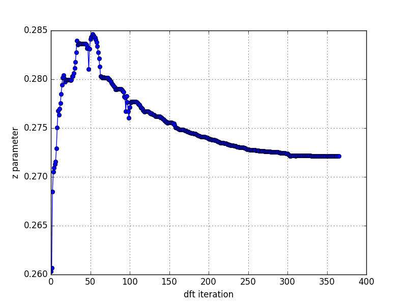
or decreased by decreasing J. For physically
relevant Hund's couplings (0.7-0.9eV), the z parameter is in the range
0.265-0.28.
2.e. Spectral function plots
Next we wanted to plot the spectral function. First we need
self-energy on the real axis, therefore we will use once more the
maximum entropy method on auxiliary Green's function (as explained in
a previous tutorial), to analytically
continue the self-energy.
To reduce the MC noise, we average the self energy (sig.inp.*) files from the
last few steps by
saverage.py saverage.py sig.inp.2[5-9].1
The output is written to sig.inpx. [We could append -o
option, if we wanted to change the sig.inpx name.]
Next, create a new directory (lets call it maxent), and copy the averaged self energy
sig.inpx into it. Also copy
the maxent_params.dat file,
which contains the parameters for the analytical continuation
process:
params={'statistics': 'fermi', # fermi/bose
        'Ntau'      : 300,     # Number of time points
        'L'         : 20.0,    # cutoff frequency on real axis
        'x0'        : 0.005,   # low energy cut-off
        'bwdth'     : 0.004,   # smoothing width
        'Nw'        : 300,     # number of frequency points on real axis
        'gwidth'    : 2*15.0,  # width of gaussian
        'idg'       : 1,       # error scheme: idg=1 -> sigma=deltag ; idg=0 -> sigma=deltag*G(tau)
        'deltag'    : 0.005,   # error
        'Asteps'    : 4000,    # anealing steps
        'alpha0'    : 1000,    # starting alpha
        'min_ratio' : 0.001,   # condition to finish, what should be the ratio
        'iflat'     : 1,       # iflat=0 : constant model, iflat=1 : gaussian of width gwidth, iflat=2 : input using file model$
        'Nitt'      : 1000,    # maximum number of outside iterations
        'Nr'        : 0,       # number of smoothing runs
        'Nf'        : 40,      # to perform inverse Fourier, high frequency limit is computed from the last Nf points
  }
Perhaps the most important is mesh on the real axis, which is given by
the upper cutoff L, the low energy cutoff x0 and
Nw points. The mesh is non-uniform and more dense at low energy
(tan-mesh).
The MC error is here set to 0.004, and can be estimated from the
variation in sig.inp.? files. Notice that we do not continue
the self-energy, which would have very large error, and would not be
stable to continue analytically. We will analytically continue an auxiliary
function, as explained in a previous tutorial.
The script which does that is called maxent_run.py. We
will thus run
or in new version of the code we can execute it with mpi in parallel
mode
mpirun -n 5 maxent_run.py sig.inpx
which will run concurent maximum entropy analytic continuation for all 5 orbitals of the problem.
This creates the
self energy Sig.out on the real axis.
Note that the newer version of maxent_run.py does not
require maxent_params.dat. If this parameter file does not exists,
it will be automatically generated with some reasonable parameter
values. Of course these values can be edited and the code can than be rerun.
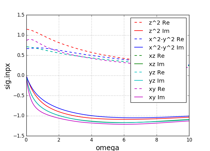
Maximum entropy should produce Sig.out, which should be similar to this plot:
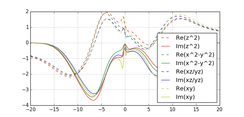 Notice that all orbitals have Fermi-liquid like behaviour at low
energy, with substantial mass enhancement. The most correlated is the
"xy" orbital. Notice also that the rotationally invariant calculation
(CoulombF="Full") would give somewhat more coherent self-energy at low
frequency, and should be preferred method of calculating
spectra. We will show this below.
Notice that all orbitals have Fermi-liquid like behaviour at low
energy, with substantial mass enhancement. The most correlated is the
"xy" orbital. Notice also that the rotationally invariant calculation
(CoulombF="Full") would give somewhat more coherent self-energy at low
frequency, and should be preferred method of calculating
spectra. We will show this below.
Now we need to make one last dmft1 calculation in order to obtain the
Green's function and DOS on the real axis. Create a new directory
inside your output directory, and while it the new directory, use
to copy necessary files from the output of the DMFT run to the new directory. Also copy the
analytically continued self energy Sig.out to sig.inp in this new
directory:
cp ../maxent/Sig.out sig.inp
Since we need to run the code on the real axis, we need to
change the NiO.indmfl file. The first number on the second line
of NiO.indmfl file determines whether the code is run on the real axis (0) or the
imaginary axis (1). Change it to 0. The header of FeSe.indmfl
file should now look like this
19 42 1 5                             # hybridization band index nemin and nemax, renormalize for interstitials, projection type
0 0.025 0.025 200 -3.000000 1.000000  # matsubara, broadening-corr, broadening-noncorr, nomega, omega_min, omega_max (in eV)
2                                     # number of correlated atoms
Then, inside the new directory run
x lapw0 -f  FeSe
x_dmft.py lapw1
x_dmft.py dmft1
mpi_prefix.dat, which contains the mpi executing command,
say mpirun -n 10, where 10 should be replaced by the
available cores on your machine. In this case one should set
OMP_NUM_THREADS=1. Alternatively, one would increase
OMP_NUM_THREADS and not use mpi_prefix.dat. In another words, these
codes have both open_MP and mpi paralleization. MPI parallelization
with respect to k-points is most efficient, but open_MP can also speed
up the execution in some parts of the code. However, using both
open_MP and mpi when we don't have enough cores available can actually
slow down the calculation.
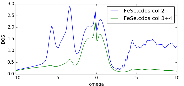
Once the run is done, we now have the densities of states on
the real axis. Both the total (column 2) and partial Fe-d (column 3
and 4)
are stored in FeSe.cdos:
Next we create a desired k-path in the Brillouin zone. One can do that
with the xcrysden tool, or, by editing a script
klist_gen.py (klist_gen.py --help should give info).
Let's create a path from Gamma, to X and to
M and back to Gamma with 240 points in total with the name FeSe.klist_band.
This can be obtained by
klist_gen.py -n 240 -p "([0,0,0],[0.5,0,0],[0.5,0.5,0],[0,0,0])" -m "['\Gamma','X','M','\Gamma']" -o FeSe.klist_band
Next, adjust the frequency range in FeSe.indmfl
file. Suppose that we want to plot spectra in the window between -1 eV
to 1 eV with 200 frequency points. The header file of
FeSe.indmfl should then be corrected to
19 42 1 5                             # hybridization band index nemin and nemax, renormalize for interstitials, projection type
0 0.025 0.025 200 -1.000000 1.000000  # matsubara, broadening-corr, broadening-noncorr, nomega, omega_min, omega_max (in eV)
Notice that we changed only the last three numbers of the second
row.
Next, in directory with real axis self-energy, run lapw on these k-points by executing
x_dmft.py lapw1 --band
x_dmft.py dmftp
The first line computes the Kohn-Sham eigenstates on the new k-points
from FeSe.klist_band. The second line computes
the frequency dependent eigenvalues, and stores them to
eigvals.dat. Now we can display the spectra by executing
Note that you might need to adjust brightness by reducing the argument
to a number between 0.0-1.0, so that the excitations are clearly seen
in the picture. The newer version of the plotting script is called
plt_akplot.py, which obtains intensity by looking at the
histogram of all momentum points. By default, 97% of data is used to
obtain the color plot. If we execute
plt_akplot.py -i 0.99
we will use 99% of the values for the plot, which will make plot
dimmer. For other options, please execute plt_akplot.py --help.
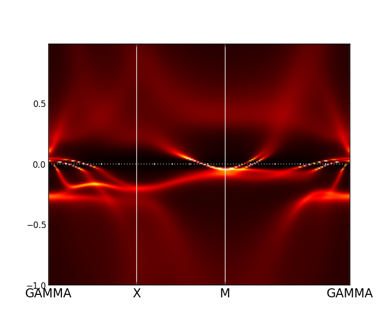
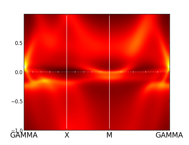 The spectra is extremely incoherent here, so that all excitations are
washed out. This is because we used quite high temperature, and
partially also
because we used density-density form of the interaction.
The spectra is extremely incoherent here, so that all excitations are
washed out. This is because we used quite high temperature, and
partially also
because we used density-density form of the interaction.
2.f. Low temperature spectra
Next, we will reduce the temperature a bit, to recover the coherence of the
spectral function. We will also use the rotationally invariant Coulomb
interaction, which should give better results (less scattering at low
energy, but higher effective masses). Note that the rotationally
invariant Coulomb interaction never leads to spin-freezing at zero
temperature. Only when the Ising interaction is used, one can get
spin-freezing down to lowest temperatures.
To proceed, we will create a new directory, and while in that directory, copy results from previous dmft run
into this new directory, i.e.,
dmft_copy.py <dmft_previous_run>
          "CoulombF"           : ["'Full'"             , "# Can be set to 'Full'"],
          "beta"               : [100                  , "# Inverse temperature"],
          "nom"                : [400                  , "# Number of Matsubara frequency points sampled"],
          "M"                  : [20e6                 , "# Total number of Monte Carlo steps"],
          "mode"               : ["SH"                 , "# We will use self-energy sampling, and Hubbard I tail"],
          "PChangeOrder"       : [0.97                 , "# How often to add/rm versus move a kink"],
          "warmup"             : [1e6                  , "# Warmup number of QMC steps"],
We will also change the mixing method back to MSR1 in
FeSe.inm file, because the structure will not change
appreciably anymore. Once we converge the solution with the full
Coulomb repulsion, using previously determined optimized structure,
the force should still be appreciably smaller than our previous cutoff
(0.5mRy/a.u.).
The first iteration is not very good, because we are starting without
status.xxx files, therefore the impurity problem starts from
atomic configuration. But nevertheless we achieve rapid convergence of
the self-energy. After a few dmft steps, we can also
increase slightly the number of MC steps, to have better statistics:
"M" : [30e6 , "# Total number of Monte Carlo steps"]
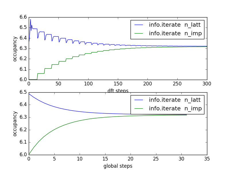
The results are converged within 5-10 DMFT steps. To have some
confidence in convergence, we will let the code run for a few more
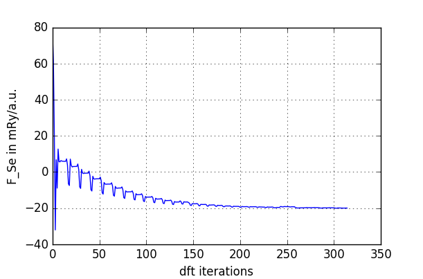
iterations. Here is the plot of total energy and free energy as a
function of dmft iterations (up to 30 dmft iterations):
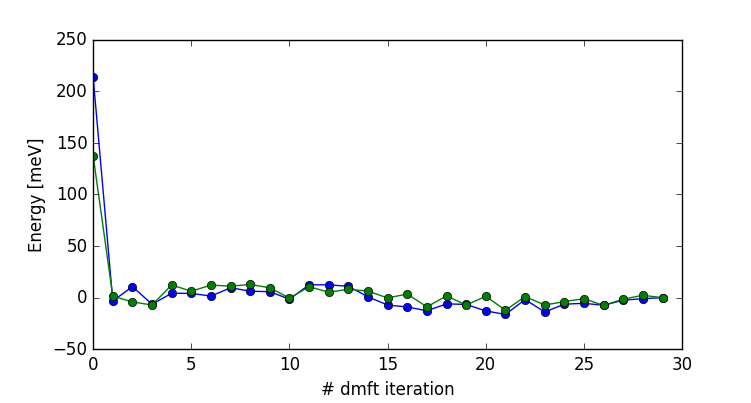 You can obtain the plot in the newer version of the code by executing
We have some MC noise, but the results seem converged after just two
iterations.
To obtain this info (printing only the dmft steps), you can also
execute
analizeInfo.py script.
You can obtain the plot in the newer version of the code by executing
We have some MC noise, but the results seem converged after just two
iterations.
To obtain this info (printing only the dmft steps), you can also
execute
analizeInfo.py script.
However, to be confident in the convergence, it is important to also
check how well is the self-energy converged. Here is the plot obtained
on 250 cores:
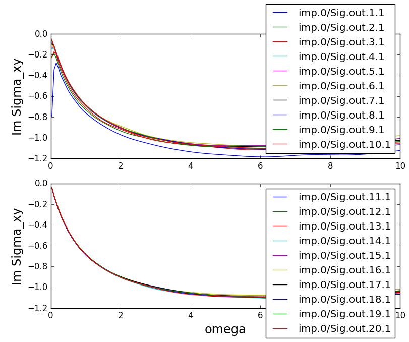 Clearly, the convergence was not good until iteration 5 or so. But
after iteration 10, the results are converged within the statistical
noise, in particular at low energy, where most of the physics is.
Clearly, the convergence was not good until iteration 5 or so. But
after iteration 10, the results are converged within the statistical
noise, in particular at low energy, where most of the physics is.
Next we will perform the analytic continuation of the self-energy. First
average self-energy over a few iterations to improve statistics:
saverage.py sig.inp.2?.1 sig.inp.30.1
 Then copy sig.inpx into a new directory for analytic
continuation, and copy maxent_params.dat from previous analytic
continuation. Finally, run
Then copy sig.inpx into a new directory for analytic
continuation, and copy maxent_params.dat from previous analytic
continuation. Finally, run
mpirun -n 5 maxent_run.py sig.inpx
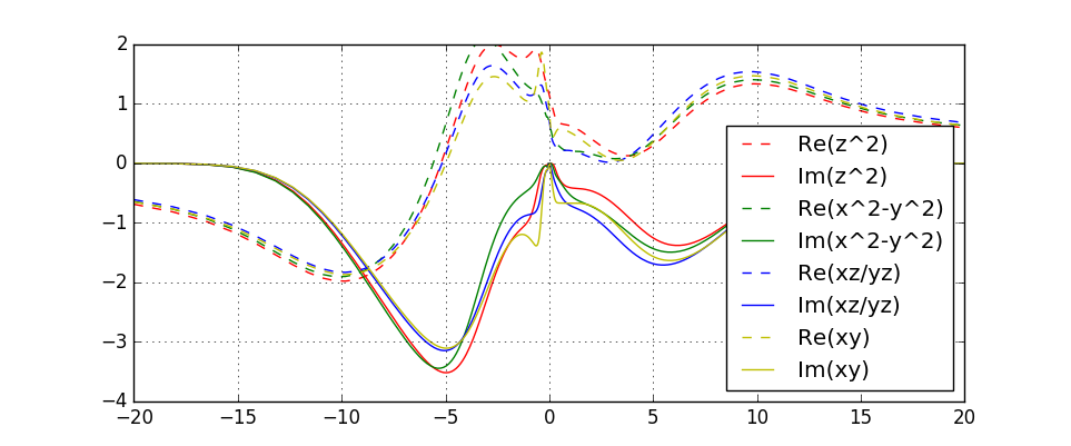 On this scale, the self-energy does not look very different from the
previous self-energy at higher temperature (and Ising-type interaction),
however, the imaginary part at zero goes to zero now, so that there is
very little scattering left at low frequency. Note that this
scattering rate can be read off from the imaginary axis data (sig.inpx) above.
On this scale, the self-energy does not look very different from the
previous self-energy at higher temperature (and Ising-type interaction),
however, the imaginary part at zero goes to zero now, so that there is
very little scattering left at low frequency. Note that this
scattering rate can be read off from the imaginary axis data (sig.inpx) above.
We will now repeat several steps from above, to obtain the density of
states on the real axis:
- create a new directory, for example on_real_axis
- while in the new director, copy converged results into the new
directory by
- in the new directory, overwrite the imaginary axis self-energy with the real axis
counterpart
cp ../maxent/Sig.out sig.inp
- Change the second line of FeSe.indmfl file, so that the
first flag (matsubara) is set to 0. Also change the frequency range
for plotting to -1.0 to 1.0, which we will need in the next
step. The second line should look like:
0 0.025 0.025 200 -1.000000 1.000000 # matsubara, broadening-corr, broadening-noncorr, nomega, omega_min, omega_max (in eV)
- Obtain DOS by running lapw0, lapw1, and dmft1 steps:
x lapw0 -f  FeSe
x_dmft.py lapw1
x_dmft.py dmft1
Not surprisingly, the DOS looks quite similar to previous results,
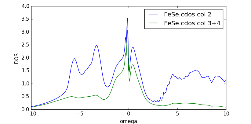 except that the quasiparticle peak is considerably sharper.
Next we copy FeSe.klist_band from previous calculation into the
current directory, and re-run Kohn-Sham diagonalization on the
selected k-path by
followed by computation of the DMFT eigenvalues
Finally display results by either
or
Notice that in the older version wakplot.py the intensity (0.1) should be tuned until a nice plot like that
 is obtained. The newer version should give nice plot by default.

2.g. Orbitally resolved spectral function
Now we want to resolve the spectra in its orbital components, i.e.,
xz, yz, and xy orbital. To do that, we will use dmftgk executable,
which can print out both the eigenvalues and the eigenvectors of the
Dyson equation. It can also be used to print k-dependent green's
function for spin susceptibility or other response function calculations.
We will first explain how to do that with the newest version of the
code, which has been streamlines, so that it is mostly automatic. Next,
we will also explain how it is done in older versions of the code,
which needs sequence of executions.
In the new version of the code one executes
This code will first check if DFT vector/energy files
correspond to high symmetry path, or regular mesh in 1BZ. It will
evaluate eDMFT eigenvectors/eigenvalues on the same mesh. This is done
in two steps: (i) first we call dmft1 in
mode "u" to print the projector. It is stored
in Udmft.??, where ?? stands for processor number. (ii) Next,
executable dmftgk is executed with mpi (uses the
same mpi_prefix.dat), and it prints eigenvalues
in eigenvalues.dat and left/right eigenvectors in UL.dat/UR.dat.
The eigenvectors are stored in large files, and it might take
substantial amount of time to combine eigenvectors from different
processors into a single file.
Once eigenvectors.dat,
UL.dat, UR.dat are available, one can display them with
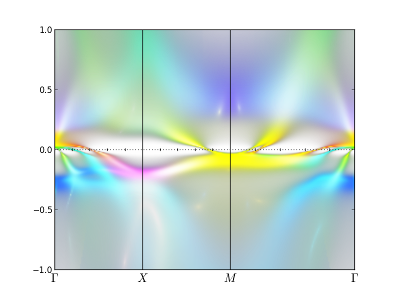
plt_sakplot.py -o "[2,2,1,1,0,2,2,1,1,0]"
The opion -o specifies the color we use for each orbital character.
We have two correlated atoms in the unit cell, which amounts to 10
orbitals, which need to be colored with one of the RGB colors. We
choose to use B for first two orbitals (the eg orbitals), G for next
two (xz & yz orbitals) and R for xy orbital. Here [0,1,2] stand for [R,G,B].
The plot should look like
 The spectral function is a
2D array of 4 numbers, first three for RGB and the forth for
transparency alpha A. The transparency is by default just the spectral
function displayed before i.e., 1/(omega+mu-ek(omega)). The colors are
the projection of the band to the choosen orbital, multiplied with the
spectral function.
We can tune darknes of the plot with overall intensity, but even more
efficiently with changing scale for colors.
With option -r we can give
a list of numbers, which are being multiplied with RGBA components of
the spectral function. For example, this command
The spectral function is a
2D array of 4 numbers, first three for RGB and the forth for
transparency alpha A. The transparency is by default just the spectral
function displayed before i.e., 1/(omega+mu-ek(omega)). The colors are
the projection of the band to the choosen orbital, multiplied with the
spectral function.
We can tune darknes of the plot with overall intensity, but even more
efficiently with changing scale for colors.
With option -r we can give
a list of numbers, which are being multiplied with RGBA components of
the spectral function. For example, this command
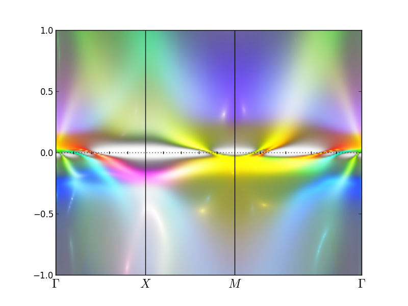
plt_sakplot.py -o "[2,2,1,1,0,2,2,1,1,0]" -r "[0.5,0.5,0.5,2]"
darkens the plot:
 it increases A, and reduces RGB.
Finally, let us comment that the two inner hole pockets around Gamma point
are primarily of xz/yz character, and the outer of xy character, since
it is red. One electron pockets at M is an equal mixture of xz/yz and
xy, since it is of yellow color (R+G). The other is more red, hence
xy. The blue color stands for eg
orbitals, which are at higher energy.
it increases A, and reduces RGB.
Finally, let us comment that the two inner hole pockets around Gamma point
are primarily of xz/yz character, and the outer of xy character, since
it is red. One electron pockets at M is an equal mixture of xz/yz and
xy, since it is of yellow color (R+G). The other is more red, hence
xy. The blue color stands for eg
orbitals, which are at higher energy.
In the next few paragraphs we explain how is the same plot
obtained in the earlier versions of the code. Note that the same
procedure can be followed with the new version of the code, but
there are two important improvements in the new version:
x_dmft.py dmftgk prints the projector and next it executed dmftgk
which uses the projector, and automatically prepares all necessary input filesdmftgk is now parallelized, and is compatible with
parallelization of dmftu step. So the execution is much faster.
2.h. Orbitally resolved spectra (dmftgk) in the older versions of the code
First, we will print DMFT projector, which relates the Fe-orbitals
with the Kohn-Sham orbitals.
x_dmft.py dmftu -g --band
The self-energy on real axis, with the desired frequency range, should normally
be prepared here. However, since we already run x_dmft.py
dmftp above, we should have files like sig.inp1_band
already present.
Next, we will prepare an input file
dmftgke.in, which should look like:
e                   # mode [g/e]: we use mode to compute eigenvalues and eigenvectors
0                   # matsubara
FeSe.energy         # LDA-energy-file, case.energy(so)(updn)
FeSe.klist_band     # k-list
FeSe.rotlm          # for reciprocal vectors
Udmft.0             # filename for projector
0.0025              # gamma for non-correlated
0.0025              # gammac
sig.inp1_band  sig.inp2_band   # self-energy name, sig.inp(x)
eigenvalues.dat     # eigenvalues
UR.dat              # right eigenvector in orbital basis
UL.dat              # left eigenvector in orbital basis
-2.                 # emin for printed eigenvalues
 2.                 # emax for printed eigenvalues
The last two lines contain the range in which the
eigenvalues/eigenvectors will be printed. Once you have
dmftgke.in file, you can execute
which prints out the eigenvalues and eigenvectors. You should see that
eigenvalues.dat, UL.dat and UR.dat appeared.
Finally, copy the python script
to your current directory, and edit it.
Scroll down to the main part of the script, which should look
something like this
if __name__ == '__main__':
    aspect_scale=0.3
    small = 1e-5
    DY = 0.0 #
    intensity = [3.,3.,3.,1.]
    COHERENCE=True
    orb_plot=[1,1,2,2,1,1,0,0,0,0,0,0,0,0] #2,2,2,2,2,2]  # should have integers 0,1,2 for red,green,blue
    #orb_plot=[]  # plotting unfolded band structure, but all orbits with hot map
To produce similar plot as before, tune
the first number in the intensity list to similar number then you
used above in wakplot.py. For example, setting
intensity = [0.1,3.,3.,1.]
will make the plot brighter. If you have much larger number of k-points
than frequency points, you might also need to tune
aspect_scale, to make plot more/less elongated. For example
will plot similar plot as wakplot.py above.
To display the plot, run
./wakplot_sophisticated.py eigenvalues.dat
First we will make two symbolic links to our eigenvectors
ln -s UL.dat UL.dat_
ln -s UR.dat UR.dat_
This is because UL.dat_ might be in general different than
UL.dat if we were attempting to unfold to a different
size Brillouin zone. We will not do that here.
Next we will tune orb_plot (in wakplot_sophisticated.py) so that different orbitals are
plotted with desired color. We have three color options, i.e., red,
green, blue, which will be assigned numbers 0,1,2. We also have 10
orbitals in total, which corresponds to 5 orbitals of the first Fe atom
and 5 of the second Fe atom, which appear in the following order
[z^2, x^2-y^2, xz, yz, xy, z^2, x^2-y^2, xz, yz, xz]. This is
of course specified in FeSe.indmfl file.
We will assign red color to xy orbital, green to xz/yz orbital and
blue to z^2 and x^2-y^2.
#         z2, x2, xz, yz, xy, z2, x2, xz, yz, xy
orb_plot=[ 2,  2,  1,  1,  0,  2,  2,  1,  1,  0]
The intensity now stands for relative intensity of the three colors
(RGB) and transparency (alpha). Lest set it to:
intensity = [3.,3.,3.,1.]
to get
 You might notice that the k-points are now displayed with Greek symbol
Gamma, rather than the text GAMMA. You can achieve that by replacing
word GAMMA in FeSe.klist_band with $\Gamma$, and M by
$M$,....
You might notice that the k-points are now displayed with Greek symbol
Gamma, rather than the text GAMMA. You can achieve that by replacing
word GAMMA in FeSe.klist_band with $\Gamma$, and M by
$M$,....
As one can see, the inside hole pocket at Gamma is almost entirely of
xz/yz character, the second pocket has a small admixture of
z^2/x^2-y^2 to the xz/yz. The outside hole pocket at Gamma is almost entirely of xy
character when it crosses the Fermi level, but it mixes with
z^2/x^2-y^2 at x-point. The electron pockets are very yellow, hence
equal mixture of xz/yz and xy character.
If we want to make the xy orbital a bit stronger, we might want to
increase the first component of intensity, or better, decrease
the second and third component of intensity. Furthermore, if we
want to make the non-Fe orbitals more transparent, we might want to
increase the last number for transparency. For example, the list
#           red,green,blue,transparent
intensity = [3.,  2.,   2.,   3.]
gives the following plot:

 and
and