Docker Tutorial: Runing eDMFT in Docker
This tutorial is useful to demonstrate several new feature in eDMFT
code, and to learn how to use twisted bilayer graphene (TBG) code. We show
three examples, MnO (which is also covered in Tutorial 1), CrSb in
magnetic state(which is not covered elsewhere) and TBG.
It is also useful to try the software without installing it
locally, or to crosscheck the local installation. It only requires
python with matplotlib (for plotting) and docker-desktop.
To install docker, please refer to these instructions for
mac,
windows,
linux.
The image name is haulek/edmftf, which is build for both the
new silicon cpu for mac (arm64) as well as intel based cpus
(amd64). The tag of the image is latest. The container is based on
linux, so during installation you might want to choose to use
primarily "Linux containers".
The installation on Mac and linux should be very straightforward.
For installation of docker on Windows, you might want to
follow the instructions here
Setting Up Docker on Windows: A Step-by-Step Guide,
or watch the video
How To Install Docker on Windows? A Step-by-Step Guide, or,
Docker Desktop for Windows 10/11 Setup and Tips.
Example 1: MnO example
Step 1: Install and Start Docker Desktop
First, install Docker Desktop locally and start the Docker application. Once
Docker Desktop is running, use the search menu to look for the image
by entering:
haulek/edmftf or edmftf
After finding the image, click on Pull to download it.
The alternative is to issue in the command prompt
docker pull haulek/edmftf:latest
This action will fetch the required image to execute eDMFT in Docker.
Note that Docker Desktop needs to be running in order to pull the image.
Step 2: Create a Directory for Output Files
Next, create an empty directory ( we will call it
examples) somewhere on your local
drive. This directory will store files generated during the Docker
run. Since graphical output is not included in this Docker, we will
plot results using Python on local machine (outside Docker).
We will copy all relevant Python
plotting scripts into this local directory to ensure accessibility
outside Docker.
Step 3: Start an Interactive Docker Session
Once the image is downloaded and the examples directory is created,
start an interactive Docker session by running the following command:
docker run -it -v ./examples:/root/examples haulek/edmftf /bin/bash
On windows this comman might need to be slightly modified:
docker run -it -v <local-path-windows-syntax>:/root/examples haulek/edmftf /bin/bash
If you get a lot of warnings on your computer, you might want to set
export FI_PROVIDER=^psm3, which switches off psm3
warnings (when occuring).
Here is what each part of the command does:
-it: Starts an interactive session.-v ./examples:/root/examples: Maps the local examples directory to /root/examples in the Docker container.haulek/edmftf: Specifies the Docker image previously pulled./bin/bash: Opens a bash shell.
If you want to only check whether the image is working, execute
docker run -it haulek/edmftf
This will not link docker files with your operating system, hence you
would not be able to see these files on your filesystem outside
docker, and plot data outside docker.
The session will start an interactive shell. In this shell, navigate
to the examples directory by executing:
cd ~/examples/
From this point onward, all commands to be executed inside the Docker
container will be shown in blue text.
Step 4: Copy Necessary Files
Copy the crystallographic information for the two examples to the current directory by running:
cp -r /app/examples/* .
This copies two examples, MnO and CrSb, as well as useful plotting
scripts to the current directory (~/examples)
For TBG example a few more plotting files are needed. If you plan to
run TBG, copy also the tbg_plt files from bin directory by:
cp /app/eDMFT/bin/tbg_plt_* .
Verify that all necessary files are present by running:
ll
The output should display:
drwxr-xr-x 3 root root    96 Jan  6 19:26 CrSb
drwxr-xr-x 3 root root    96 Jan  6 19:26 MnO
-rwxr-xr-x 1 root root  5202 Jan  6 19:26 plt_akplot.py
-rw-r--r-- 1 root root 19709 Jan  6 19:26 plt_auxiliary.py
-rwxr-xr-x 1 root root  7046 Jan  6 19:26 plt_dos.py
-rwxr-xr-x 1 root root  8865 Jan  6 19:26 plt_gs.py
-rwxr-xr-x 1 root root  1573 Jan  6 19:26 plt_info.py
-rwxr-xr-x 1 root root  6178 Jan  6 19:26 plt_makplot.py
-rwxr-xr-x 1 root root  9451 Jan  6 19:26 plt_sakplot.py
-rwxr-xr-x 1 root root  4254 Jan  6 19:26 plt_spaght.py
Step 5: Initialize the Calculation
We start with the MnO example. MnO is a charge transfer insulator in a
high-spin state with localized electrons. The Mn-d electrons will be
treated dynamically in the calculation. For this tutorial, we will set
the Coulomb interaction parameter U to 10 eV and the exchange
parameter J to 1 eV. These values are typical for transition metal oxides. They can be computed by
constrained-DMFT with supercell eDMFT calculation.
To initialize the calculation, execute the following command:
cd MnO
cif2indmf.py -U 10 -J 1 -T 100 -d 'exactd' -F 10 -f -w MnO.cif
This command converts the crystallographic MnO.cif file to a format
compatible with Wien2k (e.g., MnO.struct) and prepares all necessary
DMFT input files.
the Options are
- -U 10 -J 1: Specifies the Coulomb (Hubard and Hunds) interaction.
- -T 100: Sets the temperature to 100 K.
- -d 'exactd': Uses exact double-counting with dielectric screening, suitable for insulators like MnO.
- -F 10: Limits the calculation to a maximum of 10 self-consistent steps.
- -f: Prevents updates to the Fermi level during iterations.
- -w: Generates a momentum path for band and spectrum plotting (MnO.klist_band).
Additional Notes on Calculation Choices:
- Exact Double-Counting 'exactd' is used.
In most calculations, we use 'exacty' or 'exact' (a combination of 'exactd'
and 'exacty'). When computing exact double-counting, we construct
screened Coulomb repulsion in real space, often using a mix of
Yukawa (exacty) and dielectric (exactd) screening. Since MnO has a large charge gap,
the screening is predominantly dielectric, making exactd the most
appropriate choice.
- Convergence: The calculation stops when the change in impurity
occupancy between successive steps is less than 5e-4. This threshold
can be challenging to achieve on a laptop with limited processors, due
to Monte Carlo noise. The -F 10 option restricts the calculation to 10
impurity steps for quicker convergence.
Many DFT iterations are performed at each impurity update.
For more accuracy, this option
can be omitted to allow additional iterations.
- Chemical Potential Fixation (-f): The -f option disables Fermi
level updates at each iteration. While this speeds up convergence for
insulators like MnO, it requires verification of charge neutrality by
ensuring that the self-consistent charge density matches the valence
electron count. For charge neutrality, monitor the :DRHO entry in the
MnO.scf file. Note that the -f option should not be used for metals
and should only be applied to insulators after confirming charge
neutrality.
After these steps we should have the following files in MnO directory:
-rw-r--r-- 1 root root  4207 Dec 22 21:29 MnO.cif
-rw-r--r-- 1 root root  3812 Dec 22 21:41 MnO.struct
-rw-r--r-- 1 root root 23862 Dec 22 21:41 MnO.klist_band
-rw-r--r-- 1 root root   575 Dec 22 21:41 MnO.indmf
-rw-r--r-- 1 root root  1603 Dec 22 21:41 MnO.indmfl
-rw-r--r-- 1 root root   122 Dec 22 21:41 MnO.indmfi
-rw-r--r-- 1 root root  1942 Dec 22 21:41 params.dat
-rw-r--r-- 1 root root 79144 Dec 22 21:41 cif2struct.log
Step 6: Initialize and run DFT
Initialize the DFT calculation by running:
init_lapw
Perform the DFT self-consistent calculation:
run_lapw
This step should complete in a few minutes.
Step 7: Analyzing DFT results
To solve the Kohn-Sham problem along the high-symmetry path in the first Brillouin zone, execute:
x lapw1 -band
Next, navigate to the MnO directory on your local shell (outside Docker) and plot the resulting band structure:
../plt_spaght.py MnO.output1 -y-8:8
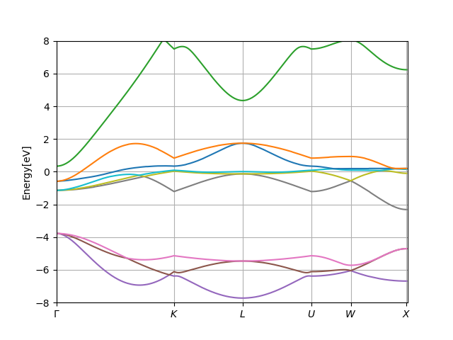
The plot will show the band structure, like that:
The plot should look like:

Note that black color commands in this tutorial should be executed outside docker, and
blue inside docker shell.
The plot shows that we have 5 bands crossing the Fermi level, which
have majority Mn:3d character. The oxygen:2p bands are found between -8eV
to -4eV, and Mn:4s state starts just above the Fermi level and is the
wide green conduction band.
Instructions for Windows users
Under Windows the plotting through python might not yet work.
First using PowerShell try to prepend the plotting command with word python, i.e.,
python ../plt_spaght.py MnO.output1 -y-8:8
If you get message that python is not installed, install it by
following your windows prompt.
If you just finished installing python, matplotlib library for plotting is
probably not included, therefore you would need to type in PowerShell
pip install matplotlib
to install matplotlib library for python, which allows plotting.
Once both python and matplotlib are in-place, you can reissue the
plotting command:
python ../plt_spaght.py MnO.output1 -y-8:8
Note that all plotting commands in PowerShell require one to
prepend python. We can omit that in unix based systems,
because the plotting scripts appear as executables.
Step 8: Initialize DMFT run
To initialize the DMFT calculation after the DFT run, execute the
following commands inside the Docker shell:
init_proj.py -a
szero.py
- init_proj.py: Calculates the radial dependence of the Mn:3d
orbitals and stores that info in projectorw.dat. This will be used
as a projector in the eDMFT calculation.
- szero.py: Creates a blank self-energy file for DMFT.
Step 9: Running and Monitoring the eDMFT Calculation
Configure parallel execution by writing the command for parallel
execution into
mpi_prefix.dat:
echo "mpirun -n 8 " > mpi_prefix.dat
Here, adjust 8 to match the number of threads your laptop supports.
Start the self-consistent eDMFT calculation:
run_dmft.py
This step may take several minutes per iteration. Monitor progress using the output files or plotting scripts.
The first impurity step is done when we see the following output:
STOP  LAPW0 END
STOP  LAPW1 END
STOP  DMFT1 END
STOP  IMPURITY_0
STOP  DMFT2 END
STOP  CORE  END
STOP  MIXER END
:ENERGY convergence: 1.0
:CHARGE convergence: 1.0
:EF     convergence: 0
:NIMP   convergence: 1
:NIMP   difference : 1

While the code is running (and after the first step is finished) we
can start plotting the progress of the calculation.
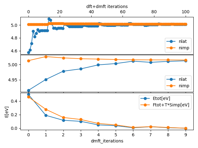
To display convergence of impurity/lattice occupancy, and total
energy, we can run (outside Docker in MnO directory):
../plt_info.py
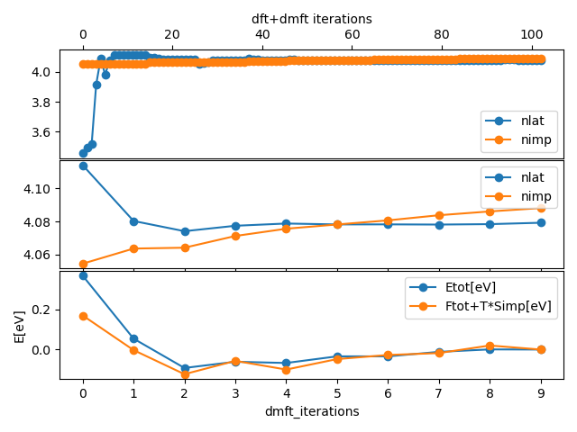
The top plot shows all DFT and DMFT steps and the Mn:5d charge as
found from impurity occupancy (nimp) and from integrating charge within muffin-tin sphere
in solid (nlat). The second plot shows the same two quantities, but
only on converged DFT charge (and each DMFT self-energy). Namely,
after impurity self-energy is recomputed, we converge DFT charge on
current self-energy. The bottom plot show the total energy and total
free energy of the system and its changes through iterations. It
should look like:

We can also monitor how similar are impurity Greens function and
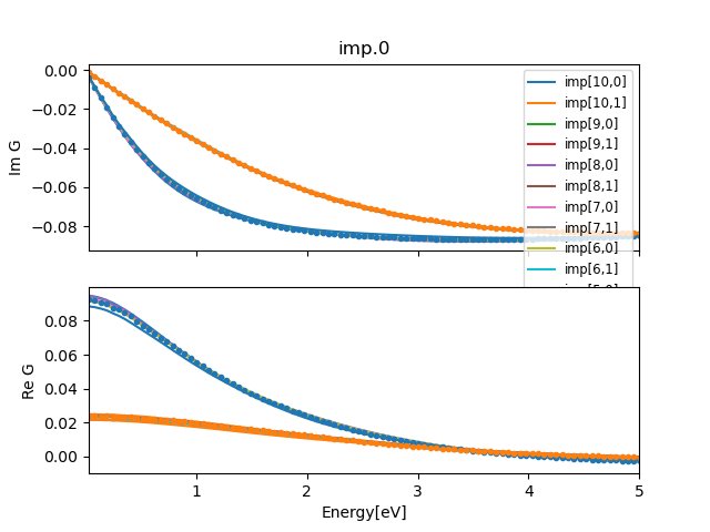
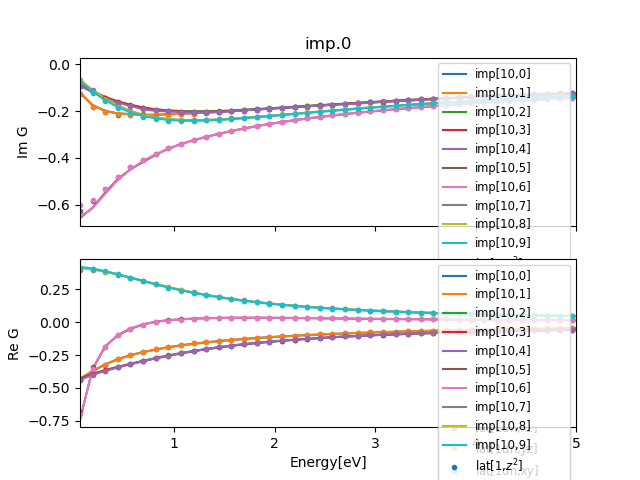
lattice Greens function. We can do that by executing
../plt_gs.py -x:5 -a 6
This plots up to 5eV frequency range, and displays last 6 impurity
Greens function. When the calculation is converged, the last impurity
Greens function should coincide with the lattice computed Greens
function. Towards the end, the plot should look like:

We see that at the beginning the current
lattice Greens function and impurity Greens function do not coincide,
but they get closer with each iteration (subject to MC noise).
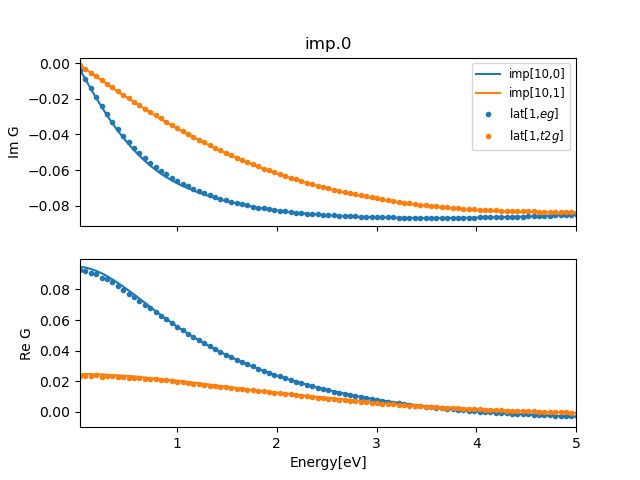
To plot the last step only, we execute:
../plt_gs.py -x:5
and if the line and dots coincide, we reached self-consistency.

The convergence is not perfect since we use only 10 steps and only 8
processors for MC calculation. But it is good enough that we can
proceed with real axis calculation.
Since we fixed the chemical potential, we need to check that the
system is charge neutral. This is achieved by
grep ':DRHO' MnO.scf
The numbers should be much smaller than unity. A unit of charge here
correspond to doping of 1 electron.
We can also monitor other files during calculation. For example:
- info.iterate : contains convergence information,
impurity/lattice occupation, total energy and free energy, etc
- MnO.dayfile: execution order and charge convergence
- dmft_info.out: information about all steps, input and output parameters
- imp.0/nohup_imp.out.000: current impurity status
- :log : summary of executions
- MnO.outputdmf1 : output from dmft1 step
- MnO.outputdmf2 : output from dmft2 step
If you need the second shell inside the docker to correct something, or to
see files that are not exposed to native shell, you can issue:
docker ps to find ID of your running docker. Thank you
can execute: docker exec -it <ID> /bin/bash.
Step 10: Real Axis Calculation and Spectral Plotting
The calculation was performed on imaginary axis, and now we want to
perform analytic continuation to the real axis, and display density of
states and the spectral function. To do that, we execute inside Docker
shell:
to_real_axis.py -y-6:6
Here -y-6:6 means that the spectral function will have frequency range
from -6eV to 6eV.
This scripts execute several steps. First the maximum entropy method
is run (inside maxent subdirectory), and than one DFT+eDMFT iteration is
performed on the real axis (inside onreal subdirectory).
We obtained density of states, the green's function on the real
axis, and the momentum resolved spectral function. To display them we execute outside the docker:
cd onreal
../../plt_gs.py -x-12:12
../../plt_dos.py -x-12:12
../../plt_akplot.py
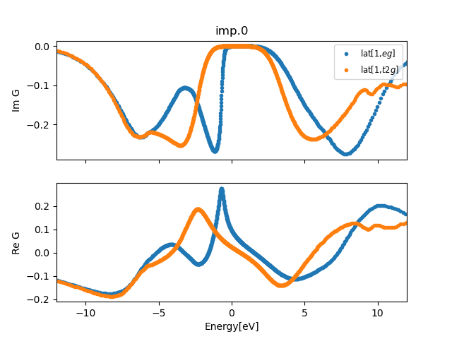
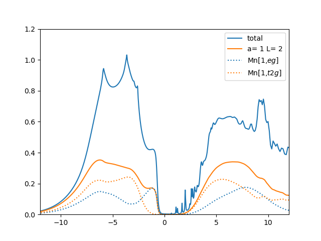
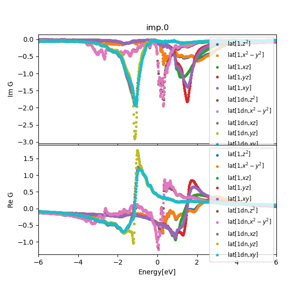
The plot of the Greens function (plt_gs.py) should produce a plot like that:

We see a clear gap of the order of 2.5eV at the Fermi level. The first
valence excitation is from eg state, which strongly hybridizes with
the oxygen below the Fermi level. The first conduction state is of t2g
origin. Interestingly, our large Coulomb repulsion of 10eV is not
clearly seen in our plot. This is because it is screened by the
oxygen:p bands and Mn:4s state, so that the Hubbard bands appear much
closer than they would in a corresponding Hubbard model.

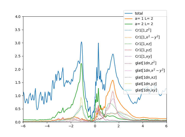
The density of states displays all states, including oxygen, and we
can see that less than 50% of the first excitation in the valence
state is of Mn:eg character, and the rest is of oxygen:2p
character. Since majority of the states just below the Fermi level are
of oxygen character, this material is characterized as charge-transfer
insulator, according to Zaanen-Sawatzky-Allen classification. The
upper Hubbard band is majority of Mn:3d character, even though there
is approximately 40% of charge that is not Mn:3d. Some is Mn:4s, and some
interstitial charge.

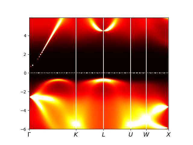
Finally, the spectral density plot (plt_akplot.py) displays the
momentum resolved spectra, which has some similarity with the DFT bands,
displayed earlier, but there are vast differences. The oxygen:p
bands, which were mostly below -4eV, are still somewhat similar,
although they move closet to EF (-3eV because of reduced level
repulsion), and became broad due to hybridization with Mn:3d. The
mixture of oxygen and Mn:3d is so-called Zhang-Rice singlet, which is
the first occupied state (between -2eV and EF), which is all that is
left from Mn:3d bands in DFT. The unoccupied Mn:4s
band is not changed much, but all the Mn:3d disappeared to
above 4eV, and is just a broad diffusive spectra, comprising the Hubbard band.
Example 2: CrSb altermagnet
Step 1: Initialize CrSb
Navigate to CrSb example directory:
cd ~/examples/CrSb
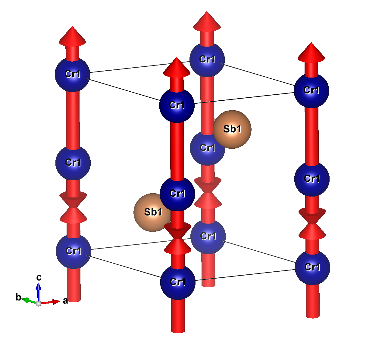
Currently we only have CrSb.mcif file, which describes its crystal
structure and magnetic configuration. It can be displayed (for
example) by VESTA, which should show:

CrSb is altermagnetic (not AFM but AM) compound that crystalizes in hexagonal space
group (194) with magnetic space group P63'/m'm'c (194.268)
More information about this material can be found at
Bilbao server.
We initialize the calculation by
cif2indmf.py -m -F 10 -w CrSb.mcif
the Options are
- -m: We want to initialize magnetic eDMFT calculation with magnetic
configuration from CrSb.mcif file
- -F 10: Limits the calculation to a maximum of 10 self-consistent steps.
- -w: Generates a momentum path for band and spectrum plotting (MnO.klist_band).
We should have the following files now:
-rw-r--r-- 1 root root  3158 Dec 22 21:29 CrSb.mcif
-rw-r--r-- 1 root root  1898 Dec 22 22:22 CrSb.struct
-rw-r--r-- 1 root root 23783 Dec 22 22:22 CrSb.klist_band
-rw-r--r-- 1 root root  1046 Dec 22 22:22 CrSb.indmf
-rw-r--r-- 1 root root  3052 Dec 22 22:22 CrSb.indmfl
-rw-r--r-- 1 root root  3052 Dec 22 22:22 CrSb.indmfldn
-rw-r--r-- 1 root root   378 Dec 22 22:22 CrSb.indmfi
-rw-r--r-- 1 root root  1942 Dec 22 22:22 params.dat
-rw-r--r-- 1 root root 37869 Dec 22 22:22 cif2struct.log
Step 2: Initialize and run DFT
Initialize the DFT calculation:
init_lapw
Perform the DFT (non-magnetic) self-consistent calculation:
run_lapw
This step should complete in a few minutes.
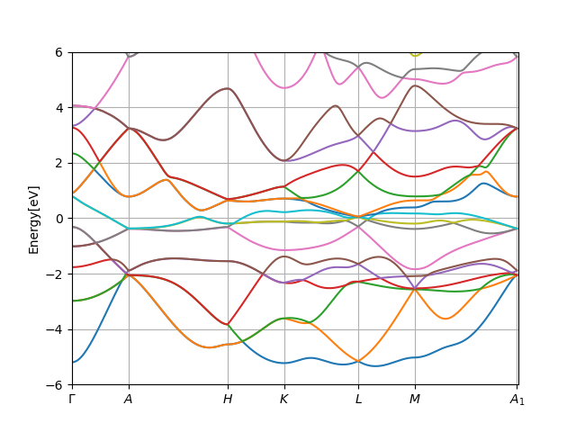
Next we check the DFT band structure by executing
x lapw1 -band
Next, navigate to the CrSb directory on your local shell (outside
Docker) and plot the resulting DFT band structure:
../plt_spaght.py CrSb.output1 -y-6:6
The plot should look like:

Step 3: Initialize and run eDMFT
Next we need to compute quasi-atomi orbital on current DFT charge
density, which is achieved by
init_proj.py -a
The blank self-energy is obtained by
szero.py -m
Here we added additional flag "-m", which adds some initial exchange
splitting to the self-energy. This should push the calculation towards
magnetic solution.
We also prepare parallel execution by
echo "mpirun -n 8 " > mpi_prefix.dat
and finally run eDMFT by
run_dmft.py
This should take approximately 40 minutes to complete 10 eDMFT steps. The
metallic systems are typically slower because the perturbation order
is larger. Indeed, we can check that average perturbation order in
hybridization expansion Monte Carlo is 290 and maximum is 450 (check "imp.0/histogram.dat").
We can monitor the convergence with (on native shell inside CrSb directory)
../plt_info.py
which should give

And as before, we can plot current Greens function by
../plt_gs.py -x:5
and should show

Notice that you can click on the legend to hide or replot each
curve. These plots have so-called dynamic legend.
Step 4: Plot results of eDMFT on real axis
Analytic continuation and plotting spectra can be achieved by one
command:
to_real_axis.py -y-6:6
Once this finishes, one can plot the green's function, density of
states and the spectral function. First navigate to
onreal directory on your native shell, and than execute
../../plt_gs.py -x-6:6
../../plt_dos.py -x-6:6
../../plt_akplot.py
which should give:


Since this is magnetic calculation the two different spin directions
do not necessary have the same spectra. In conventional AFM the
Kramers degeneracy is protected, but in altermagnets it is lifted at
least in part of momentum space. For CrSb, this is indeed the case on
xz plane, which is here achieved with the path from M to A:
../../plt_makplot.py
In most of the path the red and blue spectra coincide (Kramers
degeneracy for spin-up and spin-down). In the path from M to A the
degeneracy is lifted:

Notice that the first Brillouine zone has this form:

CrSb has lifted Kramers degeneracy in the generic point of xz (blue and green) plane,
but has degeneracy in yz (orange) plane as well as xy plane and at the
edge of BZ. Verify
that all sections of the path in above plot, except M-A, fall on planes with Kramers
degeneracy.
You can produce this plot with bz.py command.
Example 3: Twisted bilayer graphene
This example is somewhat different and demonstrates the power of
embedded DMFT idea, even when direct DFT is hard to perform. The basic model comes from
A.H. MacDonald,'s tight binding parametrization of the twisted bilayer
graphene, and the embedding DMFT idea was explained in
Haule, M., Andrei, E. Y. & Haule, K.https://arxiv.org/abs/1901.09852
(2019); and results were published in Jiang, Y. et al., Nature 573,
91-95 (2019).
Here we will reproduce the calculation from the above Nature article.
In the newer version of eDMFT code, there is a subdirectory called
tbg, which contains all the python codes for this work. The
executables are copied to your bin directory, hence they should
already be in your path. For this examples, it is important that env
variable PYTHONPATH is set to this bin directory, which should be in
variable WIEN_DMFT_ROOT. So, check that WIEN_DMFT_ROOT is set, and
that PYTHONPATH contains this directory as well.
To start, we first create new directory, say tbg, and while in that
directory, we execute:
tbg_dft.py
tbg_projector.py
The first computes the tight-binding Koh-Sham like bands for twisted
bilayer graphene, and the second computes the overlap between the
Bloch bands and the local orbitals for eDMFT calculation. The local
orbitals are defined as follows:


These four orbitals
φ0(1) ,
φ0(2),
φ0(3),
φ0(4)
are defined in real space. Their
overlap with the Bloch-bands is computed by a real space integral/sum
in tbg_projector.py. φ0(r) is a gaussian
centered on AA or AB site.
All other parameters used in the calculation are available in
tbg_params.py, which are written to the current directory. For
example, parameter par_bs['itheta']=31 selects the angle of
rotation between the two sheets of graphene. The formula for the
angle for commensurate rotations is
tan(θ/2) = 1/(2√3)/( itheta + 0.5 )
and itheta is set to 31 by default, which corresponds to angle
theta=1.05012 degrees. This is one of the magic angles. We will set a
unit in par_bs['itheta']=50, which means that we will measure all
quantities in units of 50meV. Namely, units in this example are very different
than we normally deal with, hence normalizing to an appropriate unit
of the order of unity is useful. All datafiles will hence contain
quantities in units of 50meV.
Next we set check in tbg_params.py the following two
parameters are set for plotting bands:
par['axis']='real'    # for real axis plotting
par['plt_w']=[-2.2,2.2,300]  # for frequency range -2.2*unit,2.2*unit, 300 points, here unit=50meV
tbg_dmft_scc.py
which produces so-called fat band plot, i.e., the color of bands now
depends on projection of local orbitals
φ0(1),
φ0(2),
φ0(3),
φ0(4)
to the band.
We display the fat-bands plot with:
tbg_plt_akplot.py
Note that this can not be done inside the Docker, and
tbg_plt_akplot.py should be copied to the current directory, and
executed outside the docker.

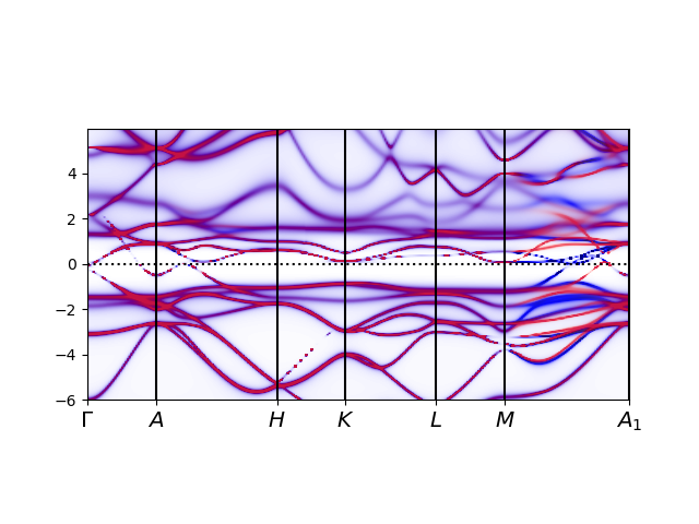
We should see a plot like above. Note that red color displays where the
four local orbitals have significant overlap with bands. As is clear,
the overlap is large for the four low energy bands, except at Gamma point,
where the character of the bands is inverted by topology.
Next we plot the partial and total density of states for this
Bloch band-structure. We first edit tbg_params.py
and set
par_bs['PlotBands'] = False
and than execute:
tbg_dft.py
tbg_projector.py
when calculation is done, we plot the density of states by
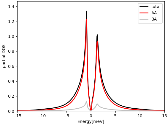
tbg_plt_dos.py -x-15:15
Here again the plotting should be done outside docker. The plot
should look like:

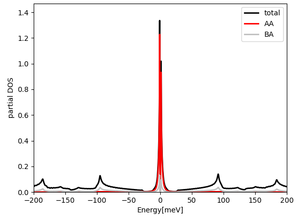
and in larger energy window:

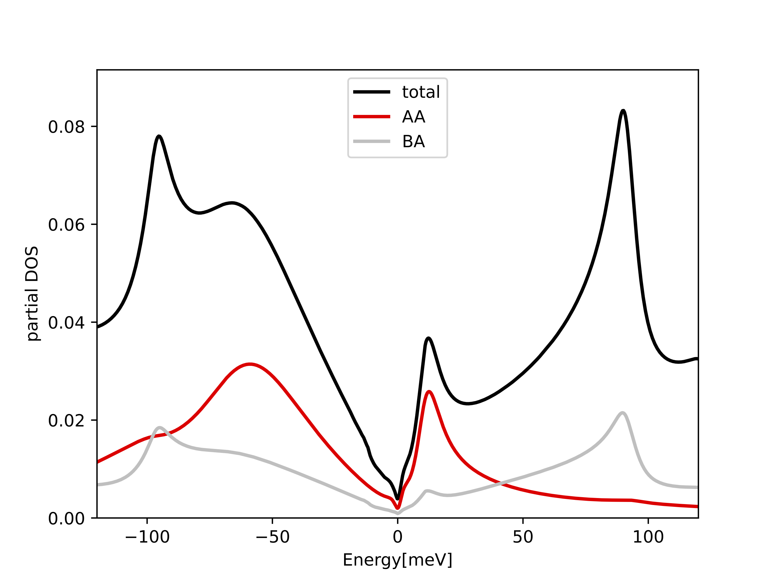
We emphasize here that the total DOS in the low energy peaks is almost
entirely contained in the projected DOS to the above orbitals centered
on the AA site (φ0(r)). Namely, when we compute the overlap in real space, we select a
gaussian of width par_pr['optimal_r'] centered on the AA site.
If we compute the overlap centered on the AB site, the overlap with
these peaks is much smaller (silver curve). If we sum the two projections up, we get
essentially 100% of total DOS within an energy windows of 3meV around
EF. This confirms that the selected real space orbitals contain all
the weight of the tight-binding model at low energy.
We can also check the hybridization of the selected orbitals with the
rest of the lattice, stored in Delta.inp. The first four
complex functions correspond to the local orbitals centered on the AA
site, and the last four to the orbitals centered on the AB site. Of
course, the hybridization of the AA-centered orbitals is small, and the
hybridization of the much more extended AB-centered orbitals is
several order of magnitude larger. We will therefore correlated only
AA-centered orbitals. The code actually correlates both, AA and AB
centered orbitals, and treats them as two independent impurity
problems. But we will not run MC for the AB-centered impurity, because
keeping self-energy at zero is a very good approximation. We will see
warnings throughout the execution:
WARNING : did not manage to read sigma from imp.1/Sigma.inp. Creating empty self-energy
which can be ignored. It says that the second impurity problem is not
being run, and hence imp.1 has vanishing self-energy.
Next we change tbg_params.py for eDMFT execution. We need
to set
par['axis']='imag'           # for imaginary axis impurity solver
Nf=<number between 0 and 8>  # set Nf occupancy
The second line sets the occupancy, which can be between 0 and 8. Namely,
we have 4 correlated orbitals, hence the maximum occupancy that can be
achieved is 8.
Next, we execute:
tbg_dmft_scc.py
to produce empty self-energy and starting hybridization on the
imaginary axis.
We than set mpi_prefix.dat for parallel execution,
for example,
echo "mpirun -n 8" > mpi_prefix.dat
and finally execute:
tbg_iterate.py
Note that these orbitals have very small hybridization compared to
their Coulomb repulsion, yet they get quite itinerant at low
energy (perturbation order is of the order of beta), hence this is
difficult to handle by hybridization expansion MC, and it requires
many processors to reduce MC noise. Nevertheless, up to some MC noise,
we can obtain reasonable approximation even on the laptop with handful
of cores. Once the 50 iterations have been completed (it might take an
hour or two), we can proceed with plotting the resulting density of
states and spectral functions.
We first create a new directory for analytic continuation, say
maxent and average over the last few steps for better
approximation to our imaginary axis self-energy
mkdir maxent
cd maxent
saverage.py -n ../imp.0/Sigma.inp.4?
maxent_run.py sig.inpx
The last command executes the maximum entropy method to get self-energy on the
real axis. We obtain Sig.out. Because the scales are
somewhat smaller in this calculation as opposed to most other
materials, we need to adjust some parameters in
maxent_params.dat. The file maxent_params.dat appears on the current
directory. We set
params["L"]=10
params["x0"]=0.002
And than we rerun maxent_run.py by
maxent_run.py sig.inpx
Once this is finished, we copy the resulting real-axis self-energy in
place of imaginary axis self-energy, i.e.,
cp Sig.out ../imp.0/Sigma.inp_real
cd ../
and we also need to change tbg_params.py for real axis
calculation:
par['axis']='real'
par['Sigma']='Sigma.inp_real'
And than we compute the density of states on the real axis by:
tbg_dmft_scc.py
and display the plot by
tbg_plt_dos.py -x-200:200
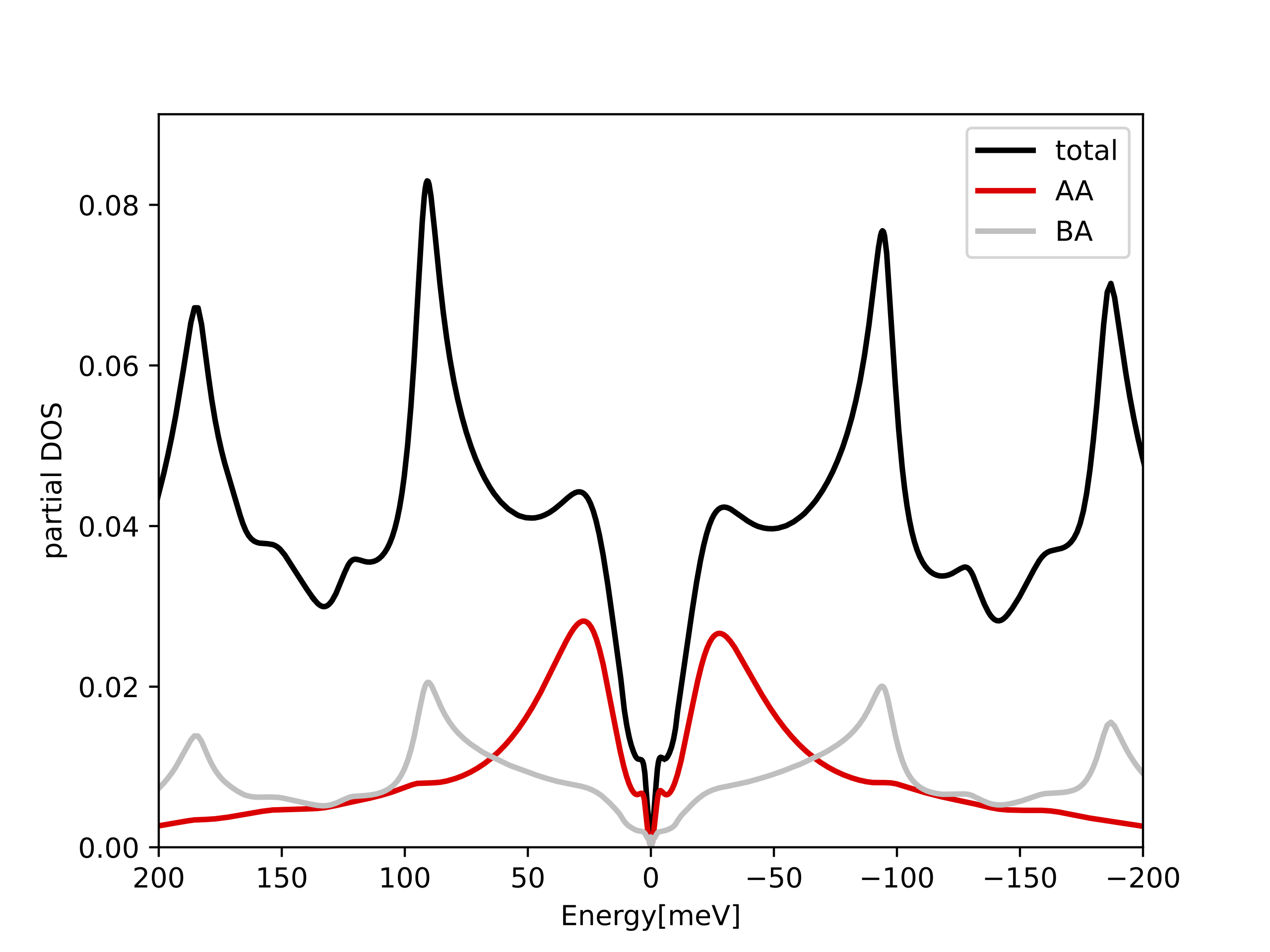
The plot for charge neutral point (Nf=4) should look like:

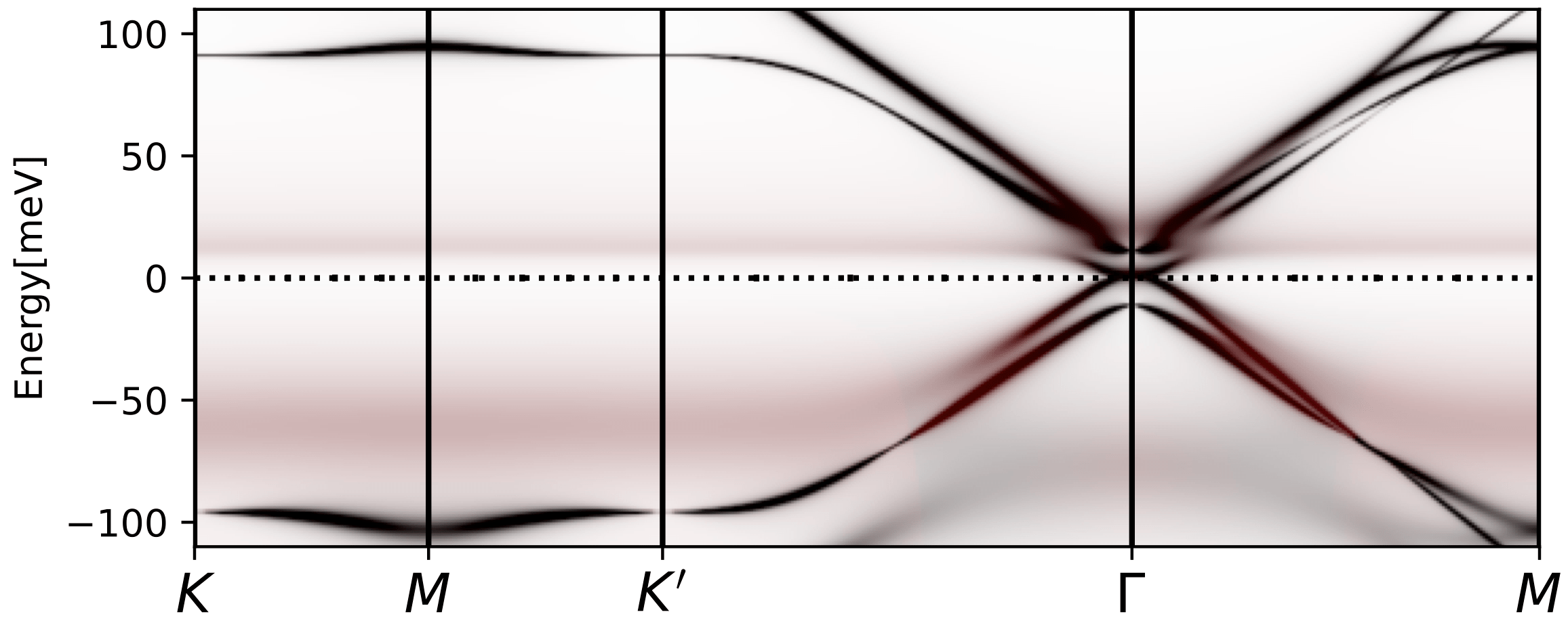
Note that the large peak at EF is transfered into the Hubbard bands,
which are located around -25meV and 25meV. Their separation is thus
50meV. Naively we would expect this scale to be U. However, the U parameter
which we used is 3*50meV=150meV (see the cited paper for details of
estimating Coulomb U). The screened interaction is thus 50meV, and is
3 times smaller than the bare U we used. It is quite common in
embedded DMFT that the Hubbard band separation is not related to
Hubbard U, but rather to emergen scale, the screened U.
Next, we change tbg_params.py one more time and set:
pars_bs['PlotBands']=True
And than we execute:
tbg_dmft_scc.py
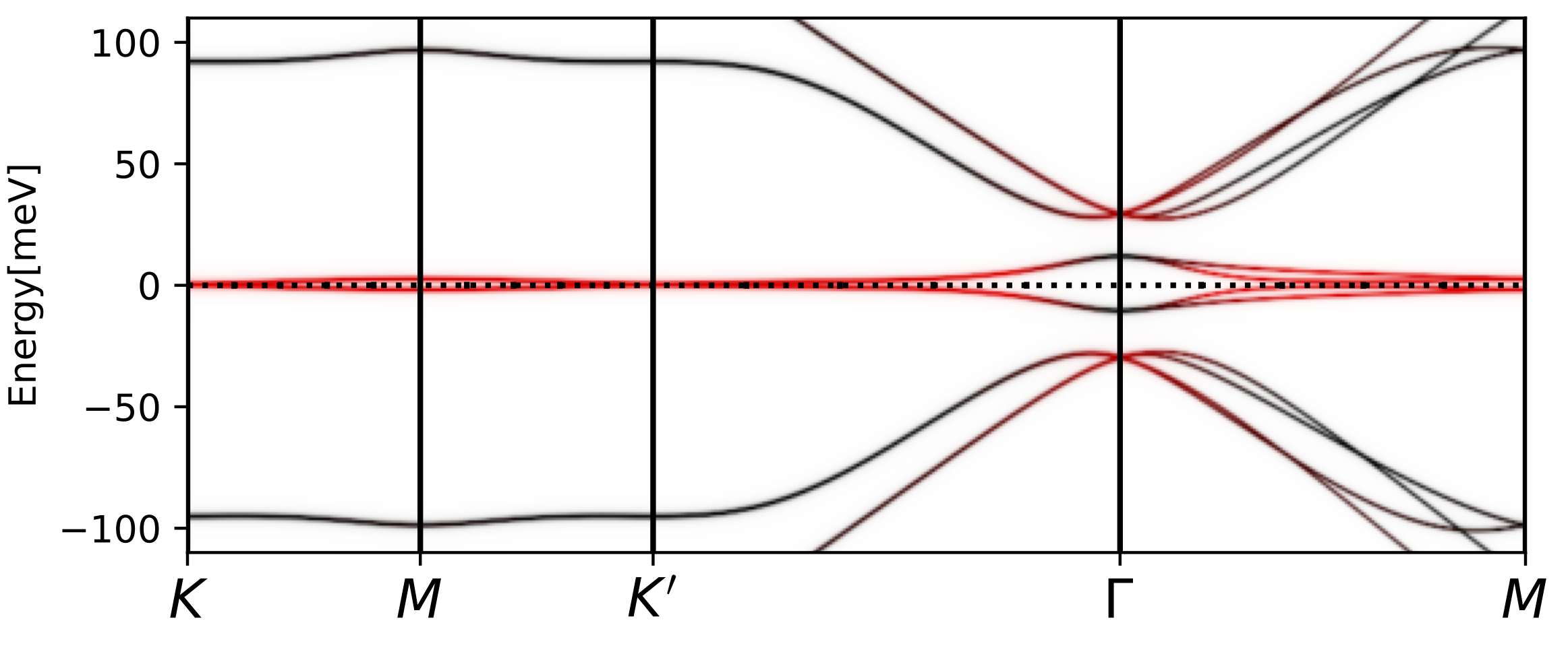
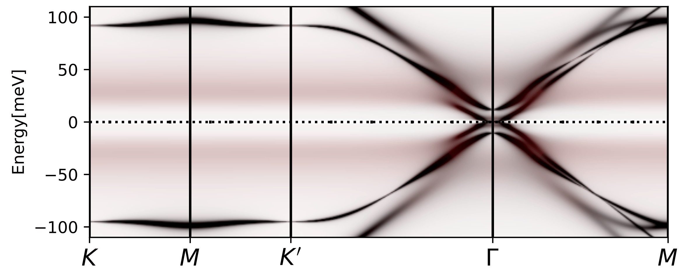
tbg_plt_akplot.py -i 0.85 -b 1e-4
We should get a plot like

The diffuse, flat in momentum, spectral weight that has red color and
is distributed between 10-50meV corresponds to the Hubbard bands we
see above. The low energy states at the Gamma point appear due to
non-trivial topology of the band structure, and can not be gapped out
by Coulomb repulsion on the AA (or AB) site. Only breaking the
symmetry can gap it out. The steep rise in the DOS above is related to
these topologically protected states that are not gapped out. These
states are very strongly scattered by the incoherent states, hence
they do not show up in transport measurement.
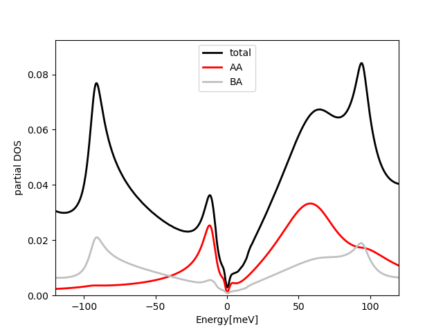
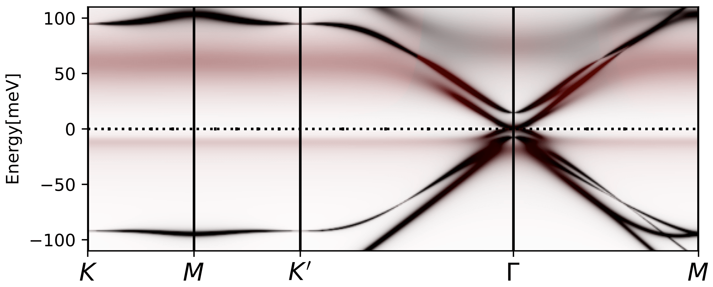
If we repeat the same calculation at filling Nf=2, which has two less
electrons than charge neutrality point, we get the following plots:


The lower Hubbard band moves closer to EF and the upper away from it,
as expected. The spectral function has similar dispersion at Gamma
point, which is left over from itinerant states, and it does not
change with doping. But the correlated bands change a lot and they are
very asymmetric.
If we change Nf to 6, we get the opposite effect, with lower Hubbard
band further from EF and upper Hubbard band closer. The spectral
function changes accordingly. The resulting plots are displayed below:
