Home What is? Install Overview CTQMC MnO FeSe SrVO3 LaVO3 Cerium Sr2IrO4 Ta2NiSe5 phonon

Tutorial 8: Lattice dynamics of FeSe

In this tutorial we will learn how to generate phonon band structure as well as other lattice dynamics properties within eDMFT. We'll obtain the phonon properties of FeSe- one of the high Tc superconductors. Some of the results have been published in Correlation driven phonon anomalies in bulk FeSe paper published in PRB.

a. Preparing the Phonon calculation job

We perform the phonon calculation using so called "frozen phonon" approximation also called "Finite displacement method". In this approximation, we generate a supercell of the crystall and then displace an atom from the symmetrically allowed position and calculate the forces on all other atoms. Before performing the phonon calculations we need to make sure the lattice structure is optimized within DMFT method and that is explained in Tutorial 2 .

The internal parameter that we optimize in FeSe is the chalcogen height (z). Once we have optimized the structure within DMFT, we proceed to generate the structures with displaced atoms allowed by symmetry of the system by using phonopy package. Please check the phonopy website for more information. Prepare a new directory and copy your optimized crystal structure file in this directory. Before we run the DMFT code, we need to generate the supercell structure which has some atoms displaced from their equilibrium position. We use the following command to generate the supercell structures.

phonopy -d --dim="2 2 2" -c FeSe.struct --wien2k

The -d arguement implies we want to generate structres with displaced atoms --dim="2 2 2" tells the code to use a 2x2x2 supercell, -c FeSe.struct gives the name of the structure file for the unit cell. --wien2k is a flag to tell the phonopy that we are using the crystal structure file in wien2k format which is .struct format.

This will generate 5 different supercell structures FeSe.structS, FeSe.structS-001, FeSe.structS-002, FeSe.structS-003, FeSe.structS-004 alongwith phonopy_disp.yaml file. We are going to run the DMFT calculations for each of FeSe.structS00x files (x=1,2,3,4). Once we have the structure files for each of the supercells, we can move forward with the DMFT calculations for each of them. For that generate 4 different directories named FeSe1, FeSe2, FeSe3, FeSe4 and copy the structure files in each of the directories respectively and rename the files to match the name of each directories. The following command would do this job if you didn't do it manually.

for i in `seq 1 4`; do mkdir FeSe${i}; cp FeSe.structS-00${i} FeSe${i}/FeSe${i}.struct; done

b. DFT initialization and self consistent run

Now we perform self consistent calculations inside each of the 4 directories that we just created- FeSe1, FeSe2, FeSe3, FeSe4. The process is exactly the same except the structure file. So we are going to show only for one of them- FeSe1.

First initialize the DFT calculation using

init_lapw

You can just enter default values for most of the inputs and use 200 k-points. The reason we are using smaller grid is that we are performing the calculation in a supercell. Once the initialization is done we need to change a flag in FeSe1.in2 file. Open the file and change the flag TOT to FOR. The first line in FeSe1.in2 file should start with FOR rather than TOT, i.e,

# FeSe1.in2, line 1 :
FOR             (TOT,FOR,QTL,EFG,FERMI)

Once the initialization is done then we submit the self consistent calculation to the cluster. Prepare teh submission script to your machine and run the self consistent DFT calculation. Since we are not trying to obtain to much of convergence within DFT we can just start with 10 lapw iterations.

c. DMFT initialization

Once the DFT self consistent run is done, we need to initialize the inputs for DMFT calculations. For thie use the script

init_dmft.py

and choose the following options:

There are 32 atoms in the unit cell:
  1 Fe
  2 Fe
  3 Fe
  4 Fe
  5 Fe
  6 Fe
  7 Fe
  8 Fe
  9 Fe
 10 Fe
 11 Fe
 12 Fe
 13 Fe
 14 Fe
 15 Fe
 16 Fe
 17 Se
 18 Se
 19 Se
 20 Se
 21 Se
 22 Se
 23 Se
 24 Se
 25 Se
 26 Se
 27 Se
 28 Se
 29 Se
 30 Se
 31 Se
 32 Se
Specify correlated atoms (ex: 1-4,7,8): 1-16
You have chosen the following atoms to be correlated:
  1 Fe
  2 Fe
  3 Fe
  4 Fe
  5 Fe
  6 Fe
  7 Fe
  8 Fe
  9 Fe
 10 Fe
 11 Fe
 12 Fe
 13 Fe
 14 Fe
 15 Fe
 16 Fe
Do you want to continue; or edit again? (c/e): c

For each atom, specify correlated orbital(s) (ex: d,f):
  1  Fe-1 d
  2  Fe-2 d
  3  Fe-3 d
  4  Fe-4 d
  5  Fe-5 d
  6  Fe-6 d
  7  Fe-7 d
  8  Fe-8 d
  9  Fe-9 d
 10  Fe-10 d
 11  Fe-11 d
 12  Fe-12 d
 13  Fe-13 d
 14  Fe-14 d
 15  Fe-15 d
 16  Fe-16 d
You have chosen to apply correlations to the following orbitals:
  1  Fe-1 d
  2  Fe-2 d
  3  Fe-3 d
  4  Fe-4 d
  5  Fe-5 d
  6  Fe-6 d
  7  Fe-7 d
  8  Fe-8 d
  9  Fe-9 d
 10  Fe-10 d
 11  Fe-11 d
 12  Fe-12 d
 13  Fe-13 d
 14  Fe-14 d
 15  Fe-15 d
 16  Fe-16 d
Do you want to continue; or edit again? (c/e): c

Specify qsplit for each correlated orbital (default = 0):
    Qsplit  Description
------  ------------------------------------------------------------
     2  real harmonics basis, no symmetry, except spin (up=dn)
------  ------------------------------------------------------------
  1  Fe-1 d: 2
  2  Fe-2 d: 2
  3  Fe-3 d: 2
  4  Fe-4 d: 2
  5  Fe-5 d: 2
  6  Fe-6 d: 2
  7  Fe-7 d: 2
  8  Fe-8 d: 2
  9  Fe-9 d: 2
 10  Fe-10 d: 2
 11  Fe-11 d: 2
 12  Fe-12 d: 2
 13  Fe-13 d: 2
 14  Fe-14 d: 2
 15  Fe-15 d: 2
 16  Fe-16 d: 2
You have chosen the following qsplits:
 1  Fe-1 d: 2
  2  Fe-2 d: 2
  3  Fe-3 d: 2
  4  Fe-4 d: 2
  5  Fe-5 d: 2
  6  Fe-6 d: 2
  7  Fe-7 d: 2
  8  Fe-8 d: 2
  9  Fe-9 d: 2
 10  Fe-10 d: 2
 11  Fe-11 d: 2
 12  Fe-12 d: 2
 13  Fe-13 d: 2
 14  Fe-14 d: 2
 15  Fe-15 d: 2
 16  Fe-16 d: 2
Do you want to continue; or edit again? (c/e): c

Specify projector type (default = 2):
------  ------------------------------------------------------------
  Projector  Drscription
     5  fixed projector, which is written to projectorw.dat. You can
        generate projectorw.dat with the tool wavef.py
------  ------------------------------------------------------------
> 5
Do you want to continue; or edit again? (c/e): c

Do you want to group any of these orbitals into cluster-DMFT problems? (y/n): n

Enter the correlated problems forming each unique correlated
problem, separated by spaces (ex: 1,3 2,4 5-8): 1-16
Each set of equivalent correlated problems are listed below:


1   (Fe1 d) (Fe2 d) (Fe3 d) (Fe4 d) (Fe5 d) (Fe6 d) (Fe7 d) (Fe8 d) (Fe9 d) (Fe10 d) (Fe11 d) (Fe12 d) (Fe13 d) (Fe14 d) (Fe15 d) (Fe16 d) are equivalent.
Do you want to continue; or edit again? (c/e): c

Range (in eV) of hybridization taken into account in impurity
problems; default -10.0, 10.0: <ENTER>

Perform calculation on real; or imaginary axis? (r/i): i

Ctrl-X-C

Is this a spin-orbit run? (y/n): n

Ctrl-X-C

The init_dmft.py script generates two necessary input files, FeSe1.indmfl and FeSe1.indmfi. They connect the solid and the impurity with the DMFT engine, respectively. Please refer to previous tutorials for understanding these files. Only difference here is that the structure is a supercell so it includes 16 Fe atoms compared to 2 in the unit cell. So we need to tell the code that each of these 16 Fe atoms are correlated atoms.

Now we want to start DMFT with the minimal number of necessary files. To do this, create a new folder (with any name), and when in that folder, use the command

dmft_copy.py <dft_results_directory>

where <dft_results_directory> is the directory where the output of the DFT calculation with DMFT initialization is. This command copies the necessary files to start a DMFT calculation. These include the .struct file as well as the various Wien2K input files such as .inm, .in1, etc. The charge density file, .clmsum, is also copied. This is all we need from the initial Wien2K run, and now we proceed to create the rest of the files, needed by the DMFT calculation.

Copy the params.dat file. This file contains information about the impurity solver and additional parameteres, which appear in DFT+EDMFT. Once again refer to Tutorial 2 for more information about the params.dat file

There is only one more file that we need: A blank self energy (sig.inp) file. Generate it by the command

szero.py

d. Running the DMFT job

Now we are ready to submit the job. The executable script is

run_dmft.py

which calls all other executable. To make the code parallel, we need to prepare at least one file mpi_prefix.dat, but it is better two prepare also mpi_prefix.dat2. The first contains the parallel command used by ctqmc code, and the second is used by the dmft1 and dmft2 step. An example of creating such command is given by

echo "mpirun -np $NSLOTS" > mpi_prefix.dat

echo "mpiexec -port $port -np $NSLOTS -machinefile $TMPDIR/machines" > mpi_prefix.dat

but the precise form of the command depends on the supercomputer and its environment.

$WIEN_DMFT_ROOT/createDMFprefix.py $JOBNAME.klist mpi_prefix.dat > mpi_prefix.dat2

where "$JOBNAME" should be set to wien2k case.

Before submitting the job, make sure that the computing notes have the following environmental variable specified: $WIENROOT, $WIEN_DMFT_ROOT, $SCRATCH. Also make sure that $WIENROOT and $WIEN_DMFT_ROOT are in $PATH as well as $WIEN_DMFT_ROOT is in $PYTHONPATH. Typically, the .bashrc will contain the following lines:

export WIENROOT=<wien-instalation-dir>
export WIEN_DMFT_ROOT=<dir-containing-dmft-executables>
export SCRATCH="."

It might be necessary to repeat these commands (seeting variables) also in the submit script. This of ocurse depends on the system.

Here we paste an example of the submit script for SUN Grid Engine , but different system will require different script.

#!/bin/bash
########################################################################
# SUN Grid Engine job wrapper
########################################################################
#$ -N FeSe1
#$ -pe mpi2 72
#$ -q <your_queue>
#$ -j y
#$ -M <email@your_institution>
#$ -m e
########################################################################
source $TMPDIR/sge_init.sh
########################################################################
export WIENROOT=<your_w2k_root>
export WIEN_DMFT_ROOT=<your_dmft_root>
export PATH=$PATH:$WIENROOT:$WIEN_DMFT_ROOT
export PYTHONPATH=$PYTHONPATH:.:$WIEN_DMFT_ROOT
export SCRATCH='.'

JOBNAME="FeSe1"   # must be equal to case name

mpi_prefix="mpiexec  -np $NSLOTS  -machinefile $TMPDIR/machines -port $port -env OMP_NUM_THREADS 1 -envlist SCRATCH,WIEN_DMFT_ROOT,PYTHONPATH,WIENROOT" 
echo $mpi_prefix > mpi_prefix.dat

$WIEN_DMFT_ROOT/createDMFprefix.py $JOBNAME.klist mpi_prefix.dat > mpi_prefix.dat2

$WIEN_DMFT_ROOT/run_dmft.py > nohup.dat 2>&1

rm -f $JOBNAME.vector*
find . -size 0|xargs rm

As opposed to the unit cell calculation the supercell takes longer computational time for each iterations. So be mindful of how much computing time you have on the machine as well. While the job is running on the cluster we can check the results after each iterations. The impurity and local occupancy could be plotted from info.iterate file (column 9 and 10). By executing analizeInfo.py, we get a printout of only dmft steps.

If we let the job run for another 20 or so iterations (finish=30), we can get much better estimation of the total energy and free energy. We can plot the self energy of different iterations to see if it's converged or not. You can use the following script to check the self energy convergence.

plot_sig.py

e. Post processing and phonon calculations

Once we have the converged calculations for each of the supercells (FeSe1, FeSe2, FeSe3, FeSe4), we can move to create the FORCE_SETS file required to obtain the phonon bands and dos. Create a separate directory to calculate the phonons and copy the .scf for each of the structures in this directory i.e. FeSe1.scf, FeSe2.scf, FeSe3.scf, FeSe4.scf. You should also copy FeSe.struct, phonopy_disp.yaml files. We now generate the FORCE_SETS file by using the following command

phonopy -f FeSe1.scf FeSe2.scf FeSe3.scf FeSe4.scf -c FeSe.struct --wien2k

-f flag is to generate the FORCE_SETS file and it uses the Forces obtained by the DMFT calculations for each of the displaced structure which are printed in FeSe1.scf FeSe2.scf, FeSe3.scf and FeSe4.scf.

e1. Generating the bands and dos files

Once we have the FORCE_SETS file then we can move ahead to do phonon calculations. First we need to prepare some input files for phonopy. For phonon band structure generate a file band.conf which looks like this.

ATOM_NAME = FeSe
DIM =  2 2 2
FC_SYMMETRY=.TRUE.
EIGENVECTORS = .TRUE
BAND_POINTS = 101
BAND = 0.5 0.5 0.0   0.5 0.5 0.5   0.0 0.0 0.0   0.5 0.0 0.0   0.5 0.5 0.0   0.0 0.0 0.0   0.0 0.0 0.5   0.5 0.0 0.5   0.5 0.5 0.5   0.0 0.0
BAND_LABELS= M A \Gamma X M \Gamma Z R A Z

The main parameters here are the direction of the high symmetry points through which we want to plot the phonon band structure. If we want to plot a character projected band structure then we need to have EIGENVECTORS = .TRUE.

Once that file is generated then we can calculate and plot the band structure by using the following command.

phonopy -p band.conf -c FeSe.struct --wien2k

We provide our own code to generate this plot as well which gives a nicer look to the same plot.

plot_phonons.py

You should get a plot something like the following.

To calculate the phonon density of states, generate a mesh.conf file which looks like following:

ATOM_NAME = FeSe
DIM = 2 2 2
MP=20 20 20
PDOS=1,3

Now we calculate the phonon density of states using the following command.

phonopy -p mesh.conf -c FeSe.struct --wien2k

e2. Atom projected DOS and phonon bands

In order to plot the atom resolved phonon DOS. You need to generate a new parameter file called params_phonon.dat. Which looks like the following:

params = {'path'    : './FeSe/',    # directory where the phonopy output files are present
          'total_dos' : False,        # If you want to plot total dos in the DOS plot
          'dos_only'  : True,         # Plot DOS only
          'band_dos'  : False,        # plot bands along with dos in the same figure
          'Econv'     : 1,            # unit conversion for energy axis (for meV 33.35643 for cm^-1)
          'Emin'      : 0.,           # minimum value of the energy axis
          'Emax'      : 40,           # maximum value of the energy axis
          'ylabel'    :'Energy (meV)',# label for y axis
          'figname'   : 'fig.pdf',    # figure name to save the figure
          'figsize'   : (8,4),        # figure size to save the plots (8,4) for bands and (8,3) for dos look nice
          'atom_type' : [0, 0, 1, 1], # indices for each atom in the system
          'atom_name' : ['Fe', 'Fe', 'Se', 'Se'] # name of the atoms in the same order as atom_type
          }

Here is a short explanation for the variables in the params.dat file. Below we explain the meaning of the variables

```
    'path'    : './FeSe/'
  
```
'path' refers to the directory where your phonon results are present.
```
    'total_dos' : False
  
```
'total_dos' takes a boolean value True/False. If True the DOS plot will also include Total DOS.
```
    'dos_only'  : True
    
```
'dos_only' takes Boolean values (True/False). If True the code only plots atom resolved phonon density of states.
```
    'band_dos'  : False
    
```
True/False. If True returns a plot with both atom resolved phonon dispersion along with density of states in the same figure. \textbf{Note:} If both 'dos_only' and 'band_dos' are False the code plots phonon bands only.
```
    Econv : 1
    
```
Unit conversion factor for energy axis. 1 => meV
```
    Emin(Emax) : 0(40)
    
```
Emin(Emax) is the minimum(maximum) values of the Energy axis in your plot. This number is multiplied by the unit conversion defined above.
```
    'ylabel'    :'Energy (meV)'
    
```
Label for the Energy axis in the plot.
```
    'figname'   : 'fig.pdf'
    
```
name of the file to save the plot.
```
    'figsize'   : (8,4)
    
```
figure size to save the plots (8,4) for bands and (8,3) for dos look nice.
```
    'atom_type' : [0, 0, 1, 1]
    
```
indices for each atom in the system as present in the structure file (POSCAR, case.struct)

    'atom_name' : ['Fe', 'Fe', 'Se', 'Se']

name of the atoms in the same order as atom_type

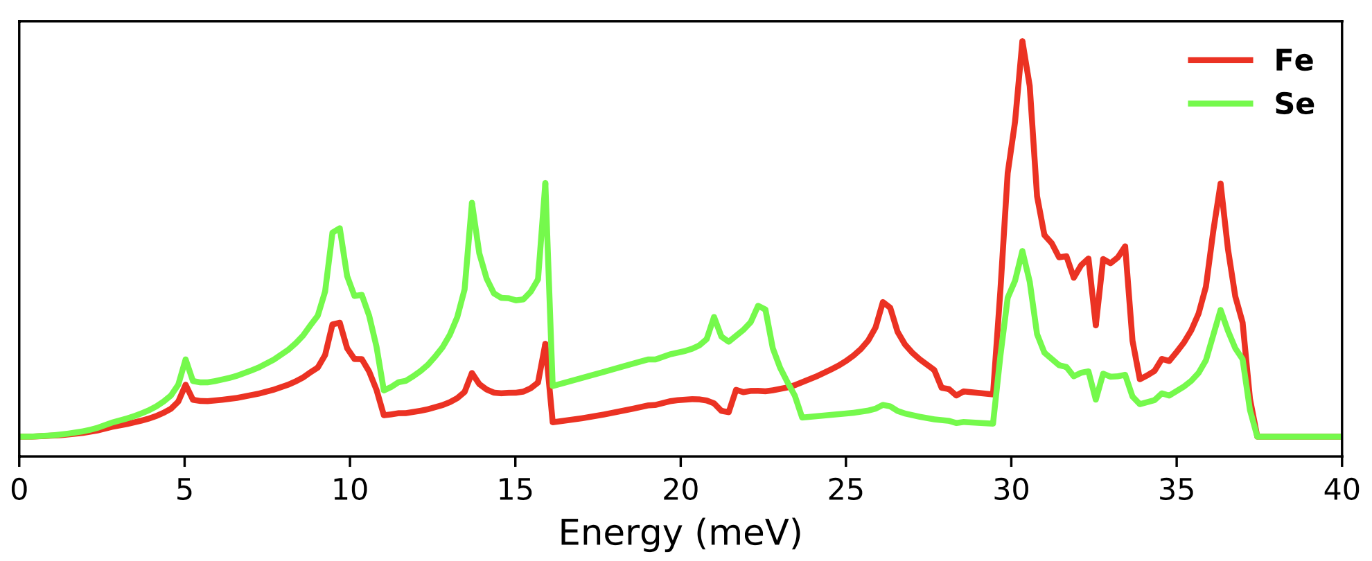
To plot the DOS only set 'dos_only' to true and run the following command.

./plot_phonons_character.py

You should get a plot something like the following.

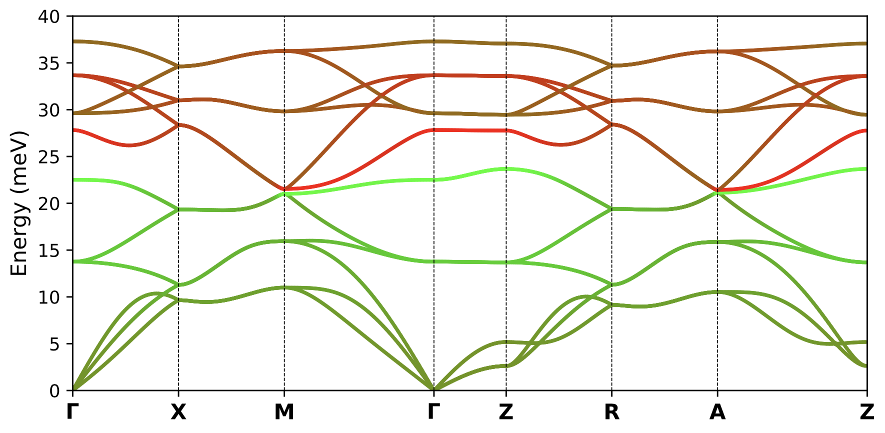
To plot the bands resolved into atomic characters, set 'dos_only' : False and 'band_dos' : False in the params_phonon.dat file and run the same command again.

./plot_phonons_character.py

This produces the following character plot.

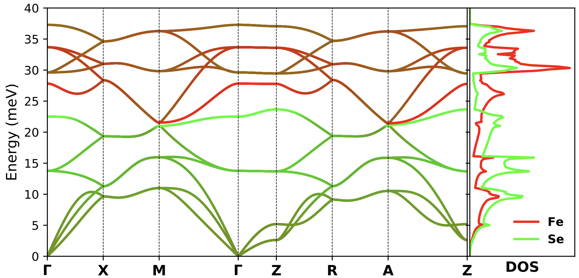
To plot the bands resolved into atomic characters as well as a DOS plot on the side, set 'dos_only' : False and 'band_dos' : True in the params_phonon.dat file and run the same command again.

./plot_phonons_character.py

You should get a plot something like the following.

Tutorial prepared by Ghanashyam Khanal and Kristjan Haule.