Home What is? Install Overview CTQMC MnO FeSe SrVO3 LaVO3 Cerium Sr2IrO4 Ta2NiSe5 phonon

Tutorial 6: Sr₂IrO₄, large spin-orbit and non-collinear magnetism

This advanced example of DFT+DMFT use will show how to set-up the run for materials with large SO and large crystal field splitting, where neither cubic harmonics nor relativistic harmonics are a very convenient basis for DMFT calculation. This tutorial will also show how to set-up antiferromagnetic calculation with non-collinear magnetic moments.

The structure file Sr2IrO4.struct is set-up for AFM calculation, it contains 8 Ir-atoms per unit cell, and two of them are inequivalent.

In the first step we set-up wien2k calculation

init_lapw

Please select non-spinpolarized calculation in wien2k. Also note that somewhat lower cut-off to separate core and valence states needs to be chosen, so that core does not leak out of the MT sphere (for example -9. would do).

Next we converge the DFT charge

run_lapw

we add spin-orbit coupling

initso

and converge the charge again

run_lapw -so

Next we increase the number of k-points (500 k-points with shifted k-mesh) and converge the charge again.

Once the DFT calculation is done, we initialize the DMFT calculation by invoking the script

init_dmft.py

We choose the following options:

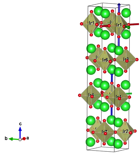
There are 56 atoms in the unit cell:
  1 Ir1
  2 Ir1
  3 Ir1
  4 Ir1
  5 Ir2
  6 Ir2
  7 Ir2
  8 Ir2
...
Specify correlated atoms (ex: 1-4,7,8): 1-8

We choose 8 Ir atom to be treated as a correlated.

For each atom, specify correlated orbital(s) (ex: d,f):
  1  Ir1-1 d
  2  Ir1-2 d
  3  Ir1-3 d
  4  Ir1-4 d
  5  Ir2-5 d
  6  Ir2-6 d
  7  Ir2-7 d
  8  Ir2-8 d

The partially filled d shell of Ir atom is to be treated in DMFT.

Specify qsplit for each correlated orbital (default = 0):
    Qsplit  Description
------  ------------------------------------------------------------
     0  average GF, non-correlated
     1  |j,mj> basis, no symmetry, except time reversal (-jz=jz)
    -1  |j,mj> basis, no symmetry, not even time reversal (-jz=jz)
     2  real harmonics basis, no symmetry, except spin (up=dn)
    -2  real harmonics basis, no symmetry, not even spin (up=dn)
     3  t2g orbitals 
    -3  eg orbitals
     4  |j,mj>, only l-1/2 and l+1/2
.....
------  ------------------------------------------------------------
  1  Ir1-1 d: 3
  2  Ir1-2 d: 3
  3  Ir1-3 d: 3
  4  Ir1-4 d: 3
  5  Ir2-5 d: 3
  6  Ir2-6 d: 3
  7  Ir2-7 d: 3
  8  Ir2-8 d: 3

We will choose to correlated the t_2g subshell.

Specify projector type (default = 2):
  Projector  Description
------  ------------------------------------------------------------
     1  projection to the solution of Dirac equation (to the head)
     2  projection to the Dirac solution, its energy derivative, 
          LO orbital, as described by P2 in PRB 81, 195107 (2010)
     4  similar to projector-2, but takes fixed number of bands in
          some energy range, even when chemical potential and 
          MT-zero moves (folows band with certain index)
     5  fixed projector, which is written to projectorw.dat. You can
        generate projectorw.dat with the tool wavef.py
------  ------------------------------------------------------------
> 5

We will again use projector 5

Do you want to group any of these orbitals into cluster-DMFT problems? (y/n): n

We do not attempt to do a cluster-DMFT calculation at this stage.

Enter the correlated problems forming each unique correlated
problem, separated by spaces (ex: 1,3 2,4 5-8): 1-8

We will use symmetry and local basis to make all atoms equivalent.

Range (in eV) of hybridization taken into account in impurity
problems; default -10.0, 10.0:  < ENTER >

This sets the energy range around the Fermi Level where hybridizations will be taken into account. Usually a value around U is a good starting guess, but one should check the resultant hybridization to see that it is enough.

Perform calculation on real; or imaginary axis? (r/i): r

We will choose real here, because we will plot partial DOS first during initialization.

Is this a spin-orbit run? (y/n): y

The spin-orbit is included.

The script init_dmft.py generates Sr2IrO4.indmfl, Sr2IrO4.indmfi and projectorw.dat. Let us take a closer look at the header of the Sr2IrO4.indmfl file:

369 832 1 5                           # hybridization band index nemin and nemax, renormalize for interstitials, projection type
0 0.025 0.025 200 -3.000000 1.000000  # matsubara, broadening-corr, broadening-noncorr, nomega, omega_min, omega_max (in eV)
8                                     # number of correlated atoms
1     1   0                           # iatom, nL, locrot
  2   3   1                           # L, qsplit, cix
2     1   0                           # iatom, nL, locrot
  2   3   2                           # L, qsplit, cix
3     1   0                           # iatom, nL, locrot
  2   3   3                           # L, qsplit, cix
4     1   0                           # iatom, nL, locrot
  2   3   4                           # L, qsplit, cix
5     1   0                           # iatom, nL, locrot
  2   3   5                           # L, qsplit, cix
6     1   0                           # iatom, nL, locrot
  2   3   6                           # L, qsplit, cix
7     1   0                           # iatom, nL, locrot
  2   3   7                           # L, qsplit, cix
8     1   0                           # iatom, nL, locrot
  2   3   8                           # L, qsplit, cix

The first two numbers in the first line specify the range of bands, which will be used for the projector (369-832). We will normalize the projector and use projector 4.

The second line shows that we are performing calculation on real axis (at the moment) and also gives k-point broadening.

Next several lines contain declaration for all 8 correlated atoms. There are two lines per atom, and the first line contains atom index, number of L-types, and locrot. This last integer (locrot) will be now changed to apply local rotations to Ir atoms, such that the local axis will coincide with octahedron cage.

The global axis of the structure is not convenient for DMFT calculation. While in principle the DMFT is rotationally invariant method, and any axis should give the same result, in practice there is enormous difference in the severity of the quamtum Monte Carlo sign problem. To minimize the sign problem, we always pick the local axis on each atom so that the hybridization matrix is maximally diagonal. This is usually the local axis, which is aligned with the local environment of the correlated atom, in this case octahedron. In this figure, we show how the local axis on Ir will be choosen below.

In the binary directory, we have a tool to find such local coordinate axis. The script is

localaxes.py

It will list a lot of information, among other all atoms in the unit cell:

  1 ATOM:  1  EQUIV.  1  Ir1        AT   0.25000   0.00000   0.87500
  2 ATOM:  1  EQUIV.  2  Ir1        AT   0.75000   0.00000   0.12500
  3 ATOM:  1  EQUIV.  3  Ir1        AT   0.75000   0.00000   0.62500
  4 ATOM:  1  EQUIV.  4  Ir1        AT   0.25000   0.00000   0.37500
  5 ATOM:  2  EQUIV.  1  Ir2        AT   0.75000   0.50000   0.37500
  6 ATOM:  2  EQUIV.  2  Ir2        AT   0.25000   0.50000   0.62500
  7 ATOM:  2  EQUIV.  3  Ir2        AT   0.25000   0.50000   0.12500
  8 ATOM:  2  EQUIV.  4  Ir2        AT   0.75000   0.50000   0.87500
.....
Enter the atom for which you want to determine local axes: 1

We will find best local axis for the first Ir-atom.

The script will find that we have octahedra, and it will calculate the local axis:

trying  cube : -N= -2.0823405461 chi2= 0.120703936262 = 3.79142326447 combined-criteria 6.71874235103
trying  octahedra : -N= -0.0823405495682 chi2= 1.48029736617e-17 = 3.79142326429 combined-criteria 0.0067799661032
trying  tetrahedra : -N= 0.0 chi2= 0.582079772951 = 3.74769905636 combined-criteria 11.4897941778
trying  square-piramid : -N= -0.0472857590573 chi2= 0.493480215373 = 3.77302040758 combined-criteria 9.743144954
According to angle variance and bond-angle we are trying octahedra with = 0.0823405495682 and = 1.48029736617e-17
Found the environment is ('octahedra', 0.082340549568209909, 1.4802973661668754e-17)

Rotation to input into case.indmfl by locrot=-1 : 

 -0.83256188   0.55393206   0.00000000 
 -0.55393206  -0.83256188   0.00000000 
  0.00000000   0.00000000   1.00000000

Let us first understand this transformation matrix. It is a unitary transformation from global cartesian coordinate system to local cartesian coordinate system. New x-axis, y-axis and z-axis are equal to the first, second and third row.

The set of atoms, which are equivalent in case.struct file, should use the same transformation to local axis. The reason is that the code will automatically find extra symmetry operation transforming first atom to any equivalent atom, and will add this extra transformation.

In our example of Sr2IrO4, we have two inequivalent atoms in structure file, and the second group of atoms starts with atom number 5. We hence need rotation for the atom nubmber 5 as well. To get it, we rerun the script

localaxes_new.py

to obtain the following rotation for atom 5:

Rotation to input into case.indmfl by locrot=-1 : 

  0.83256188  -0.55393206  -0.00000000 
 -0.55393206  -0.83256188  -0.00000000 
 -0.00000000  -0.00000000  -1.00000000

This is actually equivalent to the first rotation, hence we could also just use the first rotation for all eight atoms.

Now that we have the transformation matrix to local coordinate system, we will add it to Sr2IrO4.indmfl file. We will change locrot to -1 for the relevant atom, and paste below the transformation for that atom. The header of the Sr2IrO4.struct file will look like that

369 832 1 5                           # hybridization band index nemin and nemax, renormalize for interstitials, projection type
0 0.025 0.025 200 -3.000000 1.000000  # matsubara, broadening-corr, broadening-noncorr, nomega, omega_min, omega_max (in eV)
8                                     # number of correlated atoms
1     1  -1                           # iatom, nL, locrot
  2  14   1                           # L, qsplit, cix
 -0.83256188   0.55393206   0.00000000
 -0.55393206  -0.83256188   0.00000000
  0.00000000   0.00000000   1.00000000
2     1  -1                           # iatom, nL, locrot
  2  14   2                           # L, qsplit, cix
 -0.83256188   0.55393206   0.00000000
 -0.55393206  -0.83256188   0.00000000
  0.00000000   0.00000000   1.00000000
3     1  -1                           # iatom, nL, locrot
  2  14   3                           # L, qsplit, cix
 -0.83256188   0.55393206   0.00000000
 -0.55393206  -0.83256188   0.00000000
  0.00000000   0.00000000   1.00000000
4     1  -1                           # iatom, nL, locrot
  2  14   4                           # L, qsplit, cix
 -0.83256188   0.55393206   0.00000000
 -0.55393206  -0.83256188   0.00000000
  0.00000000   0.00000000   1.00000000
5     1  -1                           # iatom, nL, locrot
  2  14   5                           # L, qsplit, cix
  0.83256188  -0.55393206  -0.00000000
 -0.55393206  -0.83256188  -0.00000000
 -0.00000000  -0.00000000  -1.00000000
6     1  -1                           # iatom, nL, locrot
  2  14   6                           # L, qsplit, cix
  0.83256188  -0.55393206  -0.00000000
 -0.55393206  -0.83256188  -0.00000000
 -0.00000000  -0.00000000  -1.00000000
7     1  -1                           # iatom, nL, locrot
  2  14   7                           # L, qsplit, cix
  0.83256188  -0.55393206  -0.00000000
 -0.55393206  -0.83256188  -0.00000000
 -0.00000000  -0.00000000  -1.00000000
8     1  -1                           # iatom, nL, locrot
  2  14   8                           # L, qsplit, cix
  0.83256188  -0.55393206  -0.00000000
 -0.55393206  -0.83256188  -0.00000000
 -0.00000000  -0.00000000  -1.00000000

Next, we want to optimize the local rotation, so that the hybridization function is maximally diagonal. To do that, we need to run dmft1 step once (preferably on real axis, to see partial DOS).

We already removed the e_g states from correlated subset, as the Sigind and Transformation matrix take the form:

#================ # Siginds and crystal-field transformations for correlated orbitals ================
8    10   3       # Number of independent kcix blocks, max dimension, max num-independent-components
1    10   3       # cix-num, dimension, num-independent-components
#---------------- # Independent components are --------------
'xz' 'yz' 'xy' 'xz' 'yz' 'xy' 
#---------------- # Sigind follows --------------------------
1 0 0 0 0 0 0 0 0 0
0 2 0 0 0 0 0 0 0 0
0 0 3 0 0 0 0 0 0 0
0 0 0 1 0 0 0 0 0 0
0 0 0 0 2 0 0 0 0 0
0 0 0 0 0 3 0 0 0 0
0 0 0 0 0 0 0 0 0 0
0 0 0 0 0 0 0 0 0 0
0 0 0 0 0 0 0 0 0 0
0 0 0 0 0 0 0 0 0 0
#---------------- # Transformation matrix follows -----------
 0.00000000  0.00000000    0.70710679  0.00000000    0.00000000  0.00000000   -0.70710679  0.00000000    0.00000000  0.00000000    0.00000000  0.00000000    0.00000000  0.00000000    0.00000000  0.00000000    0.00000000  0.00000000    0.00000000  0.00000000  
 0.00000000  0.00000000    0.00000000  0.70710679    0.00000000  0.00000000    0.00000000  0.70710679    0.00000000  0.00000000    0.00000000  0.00000000    0.00000000  0.00000000    0.00000000  0.00000000    0.00000000  0.00000000    0.00000000  0.00000000  
-0.00000000 -0.70710679    0.00000000  0.00000000    0.00000000  0.00000000    0.00000000  0.00000000    0.00000000  0.70710679    0.00000000  0.00000000    0.00000000  0.00000000    0.00000000  0.00000000    0.00000000  0.00000000    0.00000000  0.00000000  
 0.00000000  0.00000000    0.00000000  0.00000000    0.00000000  0.00000000    0.00000000  0.00000000    0.00000000  0.00000000    0.00000000  0.00000000    0.70710679  0.00000000    0.00000000  0.00000000   -0.70710679  0.00000000    0.00000000  0.00000000  
 0.00000000  0.00000000    0.00000000  0.00000000    0.00000000  0.00000000    0.00000000  0.00000000    0.00000000  0.00000000    0.00000000  0.00000000    0.00000000  0.70710679    0.00000000  0.00000000    0.00000000  0.70710679    0.00000000  0.00000000  
 0.00000000  0.00000000    0.00000000  0.00000000    0.00000000  0.00000000    0.00000000  0.00000000    0.00000000  0.00000000   -0.00000000 -0.70710679    0.00000000  0.00000000    0.00000000  0.00000000    0.00000000  0.00000000    0.00000000  0.70710679  
 0.00000000  0.00000000    0.00000000  0.00000000    1.00000000  0.00000000    0.00000000  0.00000000    0.00000000  0.00000000    0.00000000  0.00000000    0.00000000  0.00000000    0.00000000  0.00000000    0.00000000  0.00000000    0.00000000  0.00000000  
 0.70710679  0.00000000    0.00000000  0.00000000    0.00000000  0.00000000    0.00000000  0.00000000    0.70710679  0.00000000    0.00000000  0.00000000    0.00000000  0.00000000    0.00000000  0.00000000    0.00000000  0.00000000    0.00000000  0.00000000  
 0.00000000  0.00000000    0.00000000  0.00000000    0.00000000  0.00000000    0.00000000  0.00000000    0.00000000  0.00000000    0.00000000  0.00000000    0.00000000  0.00000000    1.00000000  0.00000000    0.00000000  0.00000000    0.00000000  0.00000000  
 0.00000000  0.00000000    0.00000000  0.00000000    0.00000000  0.00000000    0.00000000  0.00000000    0.00000000  0.00000000    0.70710679  0.00000000    0.00000000  0.00000000    0.00000000  0.00000000    0.00000000  0.00000000    0.70710679  0.00000000

and now we want to find transformation to a new basis with more diagonal hybridization.

We first create a blank self-energy on the real axis. As we do not have params.dat file yet, we will need to give more arguments to the script:

szero.py -N 200 -L 25 -x 0.05

This will create 200 points mesh in the range of [-25eV,25eV] and the smallest point at 0.05eV. The mesh will be non-linear tan mesh.

If the vector files from previous self-consistent run are still available, you can skip the next steps. If not, we need to recalculate the vector files. Since the wien2k calculation is quite slow to run in serial mode, we will here run it in parallel. We first create a proper mpi_prefix.dat, and then execute

x lapw0 -f Sr2Iro4
x_dmft.py lapw1
x_dmft.py lapwso

Finally, we execute the dmft1 step to obtain the impurity levels and hybridization:

x_dmft.py dmft1

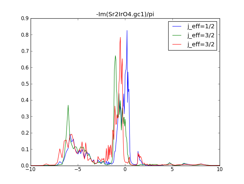
The spectral function, which is proportional to the imaginary part of the green's function from Sr2IrO4.gc1, shows doubly degenerate "xz" and "yz" states as well as the "xy" state near the Fermi level:

The dmft1 step creates Sr2IrO4.outputdmf1.0 file, which contains (at the very end of the file) the impurity levels both at infinite frequency and at low frequency. We will choose a basis in which the hybridization at low frequency is diagonal.

Automatic transformation with findRot.py

There are two ways to achieve that. We provide a script, which tries to transform to a new coordinate system automatically, and all one needs to do is to execute

findRot.py

The old file will be renamed to Sr2IrO4.indmfl_findRot and the new file Sr2IrO4.indmfl will appear, which will contain a transformation like

#================ # Siginds and crystal-field transformations for correlated orbitals ================
8    10   6       # Number of independent kcix blocks, max dimension, max num-independent-components
1    10   6       # cix-num, dimension, num-independent-components
#---------------- # Independent components are --------------
'xz' 'yz' 'xy' 'xz' 'yz' 'xy' 
#---------------- # Sigind follows --------------------------
1 0 0 0 0 0 0 0 0 0
0 2 0 0 0 0 0 0 0 0
0 0 3 0 0 0 0 0 0 0
0 0 0 4 0 0 0 0 0 0
0 0 0 0 5 0 0 0 0 0
0 0 0 0 0 6 0 0 0 0
0 0 0 0 0 0 0 0 0 0
0 0 0 0 0 0 0 0 0 0
0 0 0 0 0 0 0 0 0 0
0 0 0 0 0 0 0 0 0 0
#---------------- # Transformation matrix follows -----------
-0.00000000 -0.00000000   -0.00005873 -0.00002664   -0.00000000 -0.00000000    0.83142944 -0.00000000   -0.00000000 -0.00000000   -0.39218728 -0.02348818   -0.00000000 -0.00000000   -0.00000000 -0.00000000   -0.00000000 -0.00000000    0.39218728  0.02348818  
 0.39218727 -0.02348816    0.00000000  0.00000000    0.00000000  0.00000000    0.00000000  0.00000000   -0.39218727  0.02348816    0.00000000  0.00000000    0.83142944  0.00000000    0.00000000  0.00000000   -0.00005879  0.00002672   -0.00000000 -0.00000000  
 0.00000000  0.00000000    0.99999999  0.00000000    0.00000000  0.00000000   -0.00004935  0.00000270    0.00000000  0.00000000   -0.00012894  0.00002910    0.00000000  0.00000000    0.00000000  0.00000000    0.00000000  0.00000000    0.00012894 -0.00002910  
 0.00012888  0.00002912    0.00000000 -0.00000000   -0.00000000 -0.00000000    0.00000000 -0.00000000   -0.00012888 -0.00002912    0.00000000 -0.00000000   -0.00004924 -0.00000261   -0.00000000 -0.00000000    0.99999999 -0.00000000   -0.00000000  0.00000000  
 0.58790938 -0.00000000    0.00000000  0.00000000   -0.00000000  0.00000000    0.00000000  0.00000000   -0.58790938 -0.00000000    0.00000000  0.00000000   -0.55463656 -0.03321728   -0.00000000  0.00000000   -0.00017894  0.00003406   -0.00000000 -0.00000000  
-0.00000000  0.00000000    0.00017907  0.00003407   -0.00000000  0.00000000    0.55463657 -0.03321730   -0.00000000  0.00000000    0.58790938 -0.00000000   -0.00000000  0.00000000   -0.00000000  0.00000000   -0.00000000  0.00000000   -0.58790938  0.00000000  
 0.00000000  0.00000000    0.00000000  0.00000000    1.00000000  0.00000000    0.00000000  0.00000000    0.00000000  0.00000000    0.00000000  0.00000000    0.00000000  0.00000000    0.00000000  0.00000000    0.00000000  0.00000000    0.00000000  0.00000000  
 0.70710679  0.00000000    0.00000000  0.00000000    0.00000000  0.00000000    0.00000000  0.00000000    0.70710679  0.00000000    0.00000000  0.00000000    0.00000000  0.00000000    0.00000000  0.00000000    0.00000000  0.00000000    0.00000000  0.00000000  
 0.00000000  0.00000000    0.00000000  0.00000000    0.00000000  0.00000000    0.00000000  0.00000000    0.00000000  0.00000000    0.00000000  0.00000000    0.00000000  0.00000000    1.00000000  0.00000000    0.00000000  0.00000000    0.00000000  0.00000000  
 0.00000000  0.00000000    0.00000000  0.00000000    0.00000000  0.00000000    0.00000000  0.00000000    0.00000000  0.00000000    0.70710679  0.00000000    0.00000000  0.00000000    0.00000000  0.00000000    0.00000000  0.00000000    0.70710679  0.00000000

If you followed that route, you can now jump to section on Checking case.indmfl file

Since this script is rather new, we also explain how to obtain the same transformation in a series of steps, which the script performs.

Step by step transformation

First we find the matrix of impurity levels in Sr2IrO4.outputdmf1, which looks similar to that

 icix=           1 at omega=0
   -0.37570022     0.00000000       0.00001700    -0.18308321      -0.00000000    -0.00000000      -0.00000000     0.00000000       0.00000000     0.00000000      -0.01462619    -0.24425465   
    0.00001700     0.18308321      -0.37578835    -0.00000000      -0.00000000     0.00000000       0.00000000     0.00000000       0.00000000    -0.00000000       0.24425831    -0.01463095   
   -0.00000000     0.00000000      -0.00000000    -0.00000000      -0.47922081    -0.00000000       0.01462616     0.24425466      -0.24425827     0.01463096       0.00000000     0.00000000   
   -0.00000000    -0.00000000       0.00000000    -0.00000000       0.01462616    -0.24425466      -0.37570020    -0.00000000       0.00001704     0.18308320      -0.00000000    -0.00000000   
   -0.00000000    -0.00000000       0.00000000     0.00000000      -0.24425827    -0.01463096       0.00001704    -0.18308320      -0.37578836     0.00000000       0.00000000     0.00000000   
   -0.01462619     0.24425465       0.24425831     0.01463095       0.00000000    -0.00000000      -0.00000000     0.00000000       0.00000000    -0.00000000      -0.47922081    -0.00000000

Notice that this matrix is the same for all 8 atoms, hence we just need to deal with a single transformation.

Next, we create an input file, which will contain two matrices: i) the matrix of impurity levels, which we just found in Sr2IrO4.outputdmf1 and ii) the current transformation from spheric to cubic harmonics, which is written in Sr2IrO4.indmfl. We will name the input file diag_params.dat and it will look like that

strHc=""" 
   -0.37536788     0.00000000       0.00000523    -0.18586706       0.00003407     0.00000168       0.00000000     0.00000000      -0.00001470    -0.00001043      -0.37735904    -0.02945573   
    0.00000523     0.18586706      -0.37537965    -0.00000000      -0.00002855    -0.00000926       0.00001470     0.00001043       0.00000000     0.00000000       0.02945245    -0.37735839   
    0.00003407    -0.00000168      -0.00002855     0.00000926      -0.73087107    -0.00000000      -0.37735902    -0.02945575       0.02945245    -0.37735838      -0.00000000    -0.00000000   
    0.00000000    -0.00000000       0.00001470    -0.00001043      -0.37735902     0.02945575      -0.37536738    -0.00000000       0.00000524     0.18586689      -0.00003407     0.00000168   
   -0.00001470     0.00001043       0.00000000    -0.00000000       0.02945245     0.37735838       0.00000524    -0.18586689      -0.37537917     0.00000000       0.00002855    -0.00000926   
   -0.37735904     0.02945573       0.02945245     0.37735839      -0.00000000     0.00000000      -0.00003407    -0.00000168       0.00002855     0.00000926      -0.73087055     0.00000000   
"""

strT2C="""
 0.00000000 0.00000000   0.70710679 0.00000000   0.00000000 0.00000000  -0.70710679 0.00000000   0.00000000 0.00000000   0.00000000 0.00000000   0.00000000 0.00000000   0.00000000 0.00000000   0.00000000 0.00000000   0.00000000 0.00000000 
 0.00000000 0.00000000   0.00000000 0.70710679   0.00000000 0.00000000   0.00000000 0.70710679   0.00000000 0.00000000   0.00000000 0.00000000   0.00000000 0.00000000   0.00000000 0.00000000   0.00000000 0.00000000   0.00000000 0.00000000 
-0.70710679 0.00000000   0.00000000 0.00000000   0.00000000 0.00000000   0.00000000 0.00000000   0.70710679 0.00000000   0.00000000 0.00000000   0.00000000 0.00000000   0.00000000 0.00000000   0.00000000 0.00000000   0.00000000 0.00000000 
 0.00000000 0.00000000   0.00000000 0.00000000   0.00000000 0.00000000   0.00000000 0.00000000   0.00000000 0.00000000   0.00000000 0.00000000   0.70710679 0.00000000   0.00000000 0.00000000  -0.70710679 0.00000000   0.00000000 0.00000000 
 0.00000000 0.00000000   0.00000000 0.00000000   0.00000000 0.00000000   0.00000000 0.00000000   0.00000000 0.00000000   0.00000000 0.00000000   0.00000000 0.70710679   0.00000000 0.00000000   0.00000000 0.70710679   0.00000000 0.00000000 
 0.00000000 0.00000000   0.00000000 0.00000000   0.00000000 0.00000000   0.00000000 0.00000000   0.00000000 0.00000000  -0.70710679 0.00000000   0.00000000 0.00000000   0.00000000 0.00000000   0.00000000 0.00000000   0.70710679 0.00000000 
 0.00000000 0.00000000   0.00000000 0.00000000   1.00000000 0.00000000   0.00000000 0.00000000   0.00000000 0.00000000   0.00000000 0.00000000   0.00000000 0.00000000   0.00000000 0.00000000   0.00000000 0.00000000   0.00000000 0.00000000 
 0.70710679 0.00000000   0.00000000 0.00000000   0.00000000 0.00000000   0.00000000 0.00000000   0.70710679 0.00000000   0.00000000 0.00000000   0.00000000 0.00000000   0.00000000 0.00000000   0.00000000 0.00000000   0.00000000 0.00000000 
 0.00000000 0.00000000   0.00000000 0.00000000   0.00000000 0.00000000   0.00000000 0.00000000   0.00000000 0.00000000   0.00000000 0.00000000   0.00000000 0.00000000   1.00000000 0.00000000   0.00000000 0.00000000   0.00000000 0.00000000 
 0.00000000 0.00000000   0.00000000 0.00000000   0.00000000 0.00000000   0.00000000 0.00000000   0.00000000 0.00000000   0.70710679 0.00000000   0.00000000 0.00000000   0.00000000 0.00000000   0.00000000 0.00000000   0.70710679 0.00000000 
"""

This file now contains two python variables strHc and strT2C. They contain the matrix of impurity levels from Sr2IrO4.outputdmf1 and the matrix of transofrmation from Sr2IrO4.indmfl, respectively.

We then execute the python script find5dRotation.py

find5dRotation.py diag_params.dat

The output of the script is similar to that:

Rotation to input : 
-0.00000000 -0.00000000  -0.00005873 -0.00002664  -0.00000000 -0.00000000   0.83142944 -0.00000000  -0.00000000 -0.00000000  -0.39218728 -0.02348818  -0.00000000 -0.00000000  -0.00000000 -0.00000000  -0.00000000 -0.00000000   0.39218728  0.02348818 
 0.39218727 -0.02348816   0.00000000  0.00000000   0.00000000  0.00000000   0.00000000  0.00000000  -0.39218727  0.02348816   0.00000000  0.00000000   0.83142944  0.00000000   0.00000000  0.00000000  -0.00005879  0.00002672  -0.00000000 -0.00000000 
 0.00000000  0.00000000   0.99999999  0.00000000   0.00000000  0.00000000  -0.00004935  0.00000270   0.00000000  0.00000000  -0.00012894  0.00002910   0.00000000  0.00000000   0.00000000  0.00000000   0.00000000  0.00000000   0.00012894 -0.00002910 
 0.00012888  0.00002912   0.00000000 -0.00000000  -0.00000000 -0.00000000   0.00000000 -0.00000000  -0.00012888 -0.00002912   0.00000000 -0.00000000  -0.00004924 -0.00000261  -0.00000000 -0.00000000   0.99999999 -0.00000000  -0.00000000  0.00000000 
 0.58790938 -0.00000000   0.00000000  0.00000000  -0.00000000  0.00000000   0.00000000  0.00000000  -0.58790938 -0.00000000   0.00000000  0.00000000  -0.55463656 -0.03321728  -0.00000000  0.00000000  -0.00017894  0.00003406  -0.00000000 -0.00000000 
-0.00000000  0.00000000   0.00017907  0.00003407  -0.00000000  0.00000000   0.55463657 -0.03321730  -0.00000000  0.00000000   0.58790938 -0.00000000  -0.00000000  0.00000000  -0.00000000  0.00000000  -0.00000000  0.00000000  -0.58790938  0.00000000 
 0.00000000  0.00000000   0.00000000  0.00000000   1.00000000  0.00000000   0.00000000  0.00000000   0.00000000  0.00000000   0.00000000  0.00000000   0.00000000  0.00000000   0.00000000  0.00000000   0.00000000  0.00000000   0.00000000  0.00000000 
 0.70710679  0.00000000   0.00000000  0.00000000   0.00000000  0.00000000   0.00000000  0.00000000   0.70710679  0.00000000   0.00000000  0.00000000   0.00000000  0.00000000   0.00000000  0.00000000   0.00000000  0.00000000   0.00000000  0.00000000 
 0.00000000  0.00000000   0.00000000  0.00000000   0.00000000  0.00000000   0.00000000  0.00000000   0.00000000  0.00000000   0.00000000  0.00000000   0.00000000  0.00000000   1.00000000  0.00000000   0.00000000  0.00000000   0.00000000  0.00000000 
 0.00000000  0.00000000   0.00000000  0.00000000   0.00000000  0.00000000   0.00000000  0.00000000   0.00000000  0.00000000   0.70710679  0.00000000   0.00000000  0.00000000   0.00000000  0.00000000   0.00000000  0.00000000   0.70710679  0.00000000

which contains the new rotation, that diagonalizes hybridization function at low energy. The transformation has the same format as the original transformation from spheric to cubic harmonics in case.indmfl file. The rows specify new orbitals. The first two rows define j_eff=1/2 state, while the next four specify j_eff=3/2 states. The last four rows stand for e_g states. The columns specify the expansion in spheric harmonics and are ordered in the following convention

(-2,\downarrow),(-1,\downarrow),(0,\downarrow),(1,\downarrow),(2,\downarrow),(-2,\uparrow),(-1,\uparrow),(0,\uparrow),(1,\uparrow),(2,\uparrow)

This transformation should now replace the transformation matrix in Sr2IrO4.indmfl file. The latter should now have the following form

#================ # Siginds and crystal-field transformations for correlated orbitals ================
8    10   3       # Number of independent kcix blocks, max dimension, max num-independent-components
1    10   3       # cix-num, dimension, num-independent-components
#---------------- # Independent components are --------------
'xz' 'yz' 'xy' 'xz' 'yz' 'xy' 
#---------------- # Sigind follows --------------------------
1 0 0 0 0 0 0 0 0 0
0 1 0 0 0 0 0 0 0 0
0 0 2 0 0 0 0 0 0 0
0 0 0 2 0 0 0 0 0 0
0 0 0 0 3 0 0 0 0 0
0 0 0 0 0 3 0 0 0 0
0 0 0 0 0 0 0 0 0 0
0 0 0 0 0 0 0 0 0 0
0 0 0 0 0 0 0 0 0 0
0 0 0 0 0 0 0 0 0 0
#---------------- # Transformation matrix follows -----------
-0.00000000 -0.00000000   -0.00005873 -0.00002664   -0.00000000 -0.00000000    0.83142944 -0.00000000   -0.00000000 -0.00000000   -0.39218728 -0.02348818   -0.00000000 -0.00000000   -0.00000000 -0.00000000   -0.00000000 -0.00000000    0.39218728  0.02348818  
 0.39218727 -0.02348816    0.00000000  0.00000000    0.00000000  0.00000000    0.00000000  0.00000000   -0.39218727  0.02348816    0.00000000  0.00000000    0.83142944  0.00000000    0.00000000  0.00000000   -0.00005879  0.00002672   -0.00000000 -0.00000000  
 0.00000000  0.00000000    0.99999999  0.00000000    0.00000000  0.00000000   -0.00004935  0.00000270    0.00000000  0.00000000   -0.00012894  0.00002910    0.00000000  0.00000000    0.00000000  0.00000000    0.00000000  0.00000000    0.00012894 -0.00002910  
 0.00012888  0.00002912    0.00000000 -0.00000000   -0.00000000 -0.00000000    0.00000000 -0.00000000   -0.00012888 -0.00002912    0.00000000 -0.00000000   -0.00004924 -0.00000261   -0.00000000 -0.00000000    0.99999999 -0.00000000   -0.00000000  0.00000000  
 0.58790938 -0.00000000    0.00000000  0.00000000   -0.00000000  0.00000000    0.00000000  0.00000000   -0.58790938 -0.00000000    0.00000000  0.00000000   -0.55463656 -0.03321728   -0.00000000  0.00000000   -0.00017894  0.00003406   -0.00000000 -0.00000000  
-0.00000000  0.00000000    0.00017907  0.00003407   -0.00000000  0.00000000    0.55463657 -0.03321730   -0.00000000  0.00000000    0.58790938 -0.00000000   -0.00000000  0.00000000   -0.00000000  0.00000000   -0.00000000  0.00000000   -0.58790938  0.00000000  
 0.00000000  0.00000000    0.00000000  0.00000000    1.00000000  0.00000000    0.00000000  0.00000000    0.00000000  0.00000000    0.00000000  0.00000000    0.00000000  0.00000000    0.00000000  0.00000000    0.00000000  0.00000000    0.00000000  0.00000000  
 0.70710679  0.00000000    0.00000000  0.00000000    0.00000000  0.00000000    0.00000000  0.00000000    0.70710679  0.00000000    0.00000000  0.00000000    0.00000000  0.00000000    0.00000000  0.00000000    0.00000000  0.00000000    0.00000000  0.00000000  
 0.00000000  0.00000000    0.00000000  0.00000000    0.00000000  0.00000000    0.00000000  0.00000000    0.00000000  0.00000000    0.00000000  0.00000000    0.00000000  0.00000000    1.00000000  0.00000000    0.00000000  0.00000000    0.00000000  0.00000000  
 0.00000000  0.00000000    0.00000000  0.00000000    0.00000000  0.00000000    0.00000000  0.00000000    0.00000000  0.00000000    0.70710679  0.00000000    0.00000000  0.00000000    0.00000000  0.00000000    0.00000000  0.00000000    0.70710679  0.00000000  
......
......

Here we skipped the header and showed only the second part of the .indmfl file. We showed the transformation for the first atom only, while the .indmfl file has this information repeated 8-times, and all 8 occurrences need to be changed. Notice that both the transformation matrix and the Sigind index were changed. The latter needs to be changed because "find5dRotation.py" script ordered orbitals in such a way that two consecutive orbitals are degenerate in energy (the Kramers doublet). In magnetic state, this Kramars degeneracy will be lifted.

Please note that the orbitals are now doubly degenerate, and consequently there are only 3 inequivalent orbitals. The paramter "max num-independent-components" and "num-independent-components" was consequently changed from 6 to 3.

Checking case.indmfl file

Once the file Sr2IrO4.indmfl is updated, we should run once more the dmft1 step. First we will rerun

szero.py

so that the self-energy will now contain enough columns. Note that findRot.py made all 6 orbitals different, hence we need enough (1+6*2) columns in the self-energy file.

If vector file still exists, we might need to execute only the command

x_dmft.py dmft1

If not, we need to recalculate the vector files, as explained above.

The impurity levels in Sr2IrO4.outputdmf1 should now be diagonal, and they should take the form, similar to that

 icix=           1 at omega=0
    0.03859820    -0.00000000       0.00000000    -0.00000000       0.00000000     0.00000001      -0.00000000    -0.00000000      -0.00000000     0.00000000      -0.00000000    -0.00000000   
    0.00000000     0.00000000       0.03859818     0.00000000       0.00000000    -0.00000000      -0.00000000    -0.00000000       0.00000000    -0.00000000       0.00000000    -0.00000000   
    0.00000000    -0.00000001       0.00000000     0.00000000      -0.55882749    -0.00000000       0.00000000     0.00000000       0.00000000    -0.00000000       0.00000000    -0.00000000   
   -0.00000000     0.00000000      -0.00000000     0.00000000       0.00000000    -0.00000000      -0.55882748    -0.00000000      -0.00000000    -0.00000000       0.00000000     0.00000000   
   -0.00000000    -0.00000000       0.00000000     0.00000000       0.00000000     0.00000000      -0.00000000     0.00000000      -0.71048007    -0.00000000      -0.00000000     0.00000000   
   -0.00000000     0.00000000       0.00000000     0.00000000       0.00000000     0.00000000       0.00000000    -0.00000000      -0.00000000    -0.00000000      -0.71048008    -0.00000000

We ordered the orbitals in decreasing order (in energy), such that the doublet of j_eff=1/2 comes first, and j_eff=3/2 follows. The partial density of states, stored in Sr2IrO4.gc1 clearly shows that j_eff=1/2 is partially occupied, while the other two orbitals are nearly filled:

Before we submit DFT+DMFT job, we also need to correct the index table Sigind in Sr2IrO4.indmfi and Sr2IrO4.indmfl to be compatible. The automatic findRot.py script created the following index table

#---------------- # Sigind follows --------------------------
1 0 0 0 0 0 0 0 0 0
0 2 0 0 0 0 0 0 0 0
0 0 3 0 0 0 0 0 0 0
0 0 0 4 0 0 0 0 0 0
0 0 0 0 5 0 0 0 0 0
0 0 0 0 0 6 0 0 0 0
0 0 0 0 0 0 0 0 0 0
0 0 0 0 0 0 0 0 0 0
0 0 0 0 0 0 0 0 0 0
0 0 0 0 0 0 0 0 0 0

where all orbitals are different. This will be useful below for magnetic state. In the paramagnetic state we might want to treat the first two (jeff=1/2) orbitals as degenerate, and the second two (jeff=3/2) as degenerate, i.e., we expect Sigind to be

#---------------- # Sigind follows --------------------------
1 0 0 0 0 0 0 0 0 0
0 1 0 0 0 0 0 0 0 0
0 0 2 0 0 0 0 0 0 0
0 0 0 2 0 0 0 0 0 0
0 0 0 0 3 0 0 0 0 0
0 0 0 0 0 3 0 0 0 0
0 0 0 0 0 0 0 0 0 0
0 0 0 0 0 0 0 0 0 0
0 0 0 0 0 0 0 0 0 0
0 0 0 0 0 0 0 0 0 0

Now we have to correct Sr2IrO4.indmfi so that it contains the same index table, i.e.,

1   # number of sigind blocks
10   # dimension of this sigind block
1 0 0 0 0 0 0 0 0 0
0 1 0 0 0 0 0 0 0 0
0 0 2 0 0 0 0 0 0 0
0 0 0 2 0 0 0 0 0 0
0 0 0 0 3 0 0 0 0 0
0 0 0 0 0 3 0 0 0 0
0 0 0 0 0 0 0 0 0 0
0 0 0 0 0 0 0 0 0 0
0 0 0 0 0 0 0 0 0 0
0 0 0 0 0 0 0 0 0 0

We also need to change "matsubara" flag from 0 to 1 in "Sr2IrO4.indmfl" file, and create a blank self-energy file on Matsubara axis. After that, we can submit the DFT+DMFT job as before with "run_dmft.py" command.

Magnetic long range order

The setup in the previous step was good for the paramagnetic state. Here we want to perform calculation in the low temperature magnetic state, because the ordering temperature is quite high (T_n~240K).
We mentioned before that the first and the second orbital in our current setup are related by time-reversal symmetry, therefore degenerate in paramagnetic state. Similarly the third and the fourth orbital are related by time reversal symetry, and so on. In the magnetic state, we expect these pairs of orbitals to split, which will produce nonzero magnetic moment. We choose orbitals in such a way that the density matrix in paramagnetic state is almost diagonal, i.e., it should look like

Density matix=
n1 0  0  0  0  0  0
0  n1 0  0  0  0  0
0  0  n2 0  0  0  0
0  0  0  n2 0  0  0
0  0  0  0  n3 0  0
0  0  0  0  0  n4 0
0  0  0  0  0  0  n4

where n1 is the occupancy of j_eff=1/2 state, etc. Clearly we have blocks of 2x2 matrices for each orbital, which are diagonal in paramagnetic state. In the magnetic state, the symmetry is broaken and the 2x2 density matrix for each orbital will acquire a form:

n+delta*sigma_i

where delta is proportional to the magnetic moment, and sigma_i are Pauli matrices. The magnetic ordering can hence induce off-diagonal terms in density matrix and hybridization. Due to the Monte Carlo sign problem with off-diagonal terms, we will rather change the orbital basis in such a way, that the diagonal splitting of the form

n+delta*sigma_z

will create a magnetic moment in arbitrary direction, i.e., we will rotate the basis in spin space in such a way to keep the density matrix diagonal. This will allow us very efficient sampling with Monte Carlo impurity solver.

An additional complication here is that each atom has its own local basis and while the direction of the magnetic moment in this local basis is easy to read-off, it is tedious to transform the moment to global coordinate system. In order to make this simple, we can use a script that does just that. It takes information from Sr2IrO4.indmfl file and structure file, and calculates the magnetic moment for each correlated atom in global coordinate system. It gives matrices M_i (i=x,y,z), which can be used to calculate magnetic moment once the density matrix is known, with the following formula

m_i = Tr(M_i * n)

where n is the density matrix. Since we expect the density matrix n to be diagonal, it is very easy to determine the expected direction of the magnetic moment withouth actually performing the simulation.

The script is called local2global.py. First, execute it in the current directory:

local2global.py

which asks

Do you want to point magnetic moments in a new specified direction? [y/n]:n
Do you want short or long output [s/l]?  s
Resuts written to output file moments.dat .

It will produce information on orientation for the magnetic moment on each atom. For example, for atom 1 moments.dat shows

**** Correlated atom 1  *****
Mx_global=
 0.00002456 -0.00000000   -0.69844846 -0.57517063    0.00000316 -0.00000069    1.03237132 -0.65279371   -0.61663046 -0.45228908    0.00006982 -0.00005030    0.86837984 -0.57821706    0.50136566  0.33384327    0.00007464 -0.00006166    0.00003205 -0.00003646  
-0.69844846  0.57517063   -0.00002456  0.00000000    1.03237130  0.65279368   -0.00000316 -0.00000069    0.00006982  0.00005030    0.61663017 -0.45228888   -0.00007464 -0.00006166   -0.00003205 -0.00003646    0.86837999  0.57821716    0.50136576 -0.33384335  
 0.00000316  0.00000069    1.03237130 -0.65279368    0.00010713 -0.00000000    0.00002724  0.00000694    0.08928409 -0.01048992    0.00001064 -0.00000573    1.01944112  0.67879373    0.58856989 -0.39189466    0.00004411  0.00007345   -0.00002547 -0.00004240  
 1.03237132  0.65279371   -0.00000316  0.00000069    0.00002724 -0.00000694   -0.00010713 -0.00000000    0.00001064  0.00000573   -0.08928378 -0.01048972   -0.00004411  0.00007345    0.00002547 -0.00004240    1.01944113 -0.67879377    0.58856988  0.39189465  
-0.61663046  0.45228908    0.00006982 -0.00005030    0.08928409  0.01048992    0.00001064 -0.00000573    0.00003726  0.00000000    0.05313166 -0.09436968    0.00002913  0.00007843    0.00003115 -0.00000157   -0.50470155 -0.39602562   -0.32333616  0.18066224  
 0.00006982  0.00005030    0.61663017  0.45228888    0.00001064  0.00000573   -0.08928378  0.01048972    0.05313166  0.09436968   -0.00003726 -0.00000000    0.50470182 -0.39602584    0.32333630  0.18066234    0.00002913 -0.00007843    0.00003115  0.00000157  
 0.86837984  0.57821706   -0.00007464  0.00006166    1.01944112 -0.67879373   -0.00004411 -0.00007345    0.00002913 -0.00007843    0.50470182  0.39602584   -0.00001058 -0.00000000    0.00000000 -0.00000000    0.83236365 -0.55422988    0.00000000  0.00000000  
 0.50136566 -0.33384327   -0.00003205  0.00003646    0.58856989  0.39189466    0.00002547  0.00004240    0.00003115  0.00000157    0.32333630 -0.18066234    0.00000000 -0.00000000   -0.00001058  0.00000000   -0.00000000 -0.00000000    0.83236367 -0.55422989  
 0.00007464  0.00006166    0.86837999 -0.57821716    0.00004411 -0.00007345    1.01944113  0.67879377   -0.50470155  0.39602562    0.00002913  0.00007843    0.83236365  0.55422988   -0.00000000 -0.00000000    0.00001058 -0.00000000    0.00000000  0.00000000  
 0.00003205  0.00003646    0.50136576  0.33384335   -0.00002547  0.00004240    0.58856988 -0.39189465   -0.32333616 -0.18066224    0.00003115 -0.00000157    0.00000000 -0.00000000    0.83236367  0.55422989   -0.00000000 -0.00000000    0.00001058  0.00000000  
My_global=
 0.00004264 -0.00000000    0.57522388 -0.69843801    0.00000424  0.00015729   -0.65276669 -1.03237702    0.45230126 -0.61662159   -0.00011231 -0.00007644   -0.57822314 -0.86840633   -0.33382780  0.50136832   -0.00004970  0.00004105   -0.00007786  0.00001986  
 0.57522388  0.69843801   -0.00004264 -0.00000000   -0.65276668  1.03237699   -0.00000424  0.00015729   -0.00011231  0.00007644   -0.45230107 -0.61662136    0.00004970  0.00004105    0.00007786  0.00001986   -0.57822326  0.86840653   -0.33382785 -0.50136842  
 0.00000424 -0.00015729   -0.65276668 -1.03237699    0.00001265  0.00000000    0.00000695 -0.00002723   -0.01047193 -0.08928636   -0.00000106 -0.00000029   -0.67878667  1.01942512   -0.39190476 -0.58857009    0.00006624  0.00011030   -0.00003825 -0.00006368  
-0.65276669  1.03237702   -0.00000424 -0.00015729    0.00000695  0.00002723   -0.00001265  0.00000000   -0.00000106  0.00000029    0.01047170 -0.08928603   -0.00006624  0.00011030    0.00003825 -0.00006368   -0.67878664 -1.01942511   -0.39190478  0.58857011  
 0.45230126  0.61662159   -0.00011231 -0.00007644   -0.01047193  0.08928636   -0.00000106 -0.00000029    0.00000319  0.00000000   -0.09437060 -0.05312998   -0.00001247  0.00003574    0.00006745 -0.00004974    0.39602833 -0.50468873    0.18066847  0.32333186  
-0.00011231  0.00007644   -0.45230107  0.61662136   -0.00000106  0.00000029    0.01047170  0.08928603   -0.09437060  0.05312998   -0.00000319  0.00000000   -0.39602848 -0.50468901   -0.18066858  0.32333204   -0.00001247 -0.00003574    0.00006745  0.00004974  
-0.57822314  0.86840633    0.00004970 -0.00004105   -0.67878667 -1.01942512   -0.00006624 -0.00011030   -0.00001247 -0.00003574   -0.39602848  0.50468901   -0.00004707  0.00000000    0.00000000 -0.00000000   -0.55422987 -0.83236365    0.00000000 -0.00000000  
-0.33382780 -0.50136832    0.00007786 -0.00001986   -0.39190476  0.58857009    0.00003825  0.00006368    0.00006745  0.00004974   -0.18066858 -0.32333204    0.00000000  0.00000000   -0.00004707 -0.00000000    0.00000000 -0.00000000   -0.55422989 -0.83236367  
-0.00004970 -0.00004105   -0.57822326 -0.86840653    0.00006624 -0.00011030   -0.67878664  1.01942511    0.39602833  0.50468873   -0.00001247  0.00003574   -0.55422987  0.83236365    0.00000000  0.00000000    0.00004707  0.00000000   -0.00000000 -0.00000000  
-0.00007786 -0.00001986   -0.33382785  0.50136842   -0.00003825  0.00006368   -0.39190478 -0.58857011    0.18066847 -0.32333186    0.00006745 -0.00004974    0.00000000  0.00000000   -0.55422989  0.83236367    0.00000000  0.00000000    0.00004707  0.00000000  
Mz_global=
-1.17689005  0.00000000    0.00006524 -0.00006784   -0.00000217  0.00000732    0.00012145  0.00000272   -0.00005380  0.00010349   -1.33452976 -0.10416443    0.00001803  0.00004699    0.00008675 -0.00002589    0.00000000 -0.00000000   -1.04443013 -0.08152121  
 0.00006524  0.00006784    1.17689093  0.00000000    0.00012145 -0.00000272    0.00000214  0.00000737   -1.33452933  0.10416445    0.00005380  0.00010349   -0.00000000 -0.00000000    1.04442956 -0.08152121    0.00001803 -0.00004699    0.00008675  0.00002589  
-0.00000217 -0.00000732    0.00012145  0.00000272    0.00000001  0.00000000    0.00000000  0.00000000   -0.00003862  0.00004562   -0.00001023 -0.00001190    0.00002116 -0.00005517   -0.00002461  0.00002489   -0.00000000 -0.00000001   -0.00001575 -0.00001244  
 0.00012145 -0.00000272    0.00000214 -0.00000737    0.00000000 -0.00000000   -0.00000001  0.00000000   -0.00001023  0.00001193    0.00003862  0.00004562    0.00000000 -0.00000001    0.00001578 -0.00001244    0.00002116  0.00005517   -0.00002461 -0.00002489  
-0.00005380 -0.00010349   -1.33452933 -0.10416445   -0.00003862 -0.00004562   -0.00001023 -0.00001193   -0.17689092  0.00000000    0.00004316 -0.00003740    0.00000000 -0.00000000    1.70367877  0.00000000   -0.00001330  0.00002795   -0.00000508 -0.00001713  
-1.33452976  0.10416443    0.00005380 -0.00010349   -0.00001023  0.00001190    0.00003862 -0.00004562    0.00004316  0.00003740    0.17689007  0.00000000    0.00001330  0.00002795    0.00000508 -0.00001713    0.00000000  0.00000000    1.70367843 -0.00000000  
 0.00001803 -0.00004699   -0.00000000  0.00000000    0.00002116  0.00005517    0.00000000  0.00000001    0.00000000  0.00000000    0.00001330 -0.00002795   -1.00000000  0.00000000   -0.00000000  0.00000000    0.00001728  0.00004504    0.00000000  0.00000000  
 0.00008675  0.00002589    1.04442956  0.08152121   -0.00002461 -0.00002489    0.00001578  0.00001244    1.70367877 -0.00000000    0.00000508  0.00001713    0.00000000  0.00000000   -1.00000002  0.00000000   -0.00000000  0.00000000    0.00001728  0.00004504  
 0.00000000  0.00000000    0.00001803  0.00004699   -0.00000000  0.00000001    0.00002116 -0.00005517   -0.00001330 -0.00002795    0.00000000 -0.00000000    0.00001728 -0.00004504    0.00000000 -0.00000000    1.00000000  0.00000000    0.00000000  0.00000000  
-1.04443013  0.08152121    0.00008675 -0.00002589   -0.00001575  0.00001244   -0.00002461  0.00002489   -0.00000508  0.00001713    1.70367843  0.00000000    0.00000000 -0.00000000    0.00001728 -0.00004504    0.00000000 -0.00000000    1.00000002  0.00000000

Suppose that the density matrix of j_eff=1/2 has the form n=n₀I+delta*sigma_z. According to the above results, the magnetic moment in x and y direction will vanish, while in z-direction it will be equal to m_z=-1.177*2*delta. Notice that this magnetic moment is already calculated in the global coordinate system. Similarly, we can determine magnetic moment for any atom.

In Sr2IrO4 the magnetic moment is pointing in-plane, and it rotates rigidly with the oxygen octahedra. In the local coordinate system of the octahedra, it is pointing in the direction of (±1,±1,0). In global coordinate system, the moment is pointing mainly in x-direction, but it is canted for ~12 degrees due to the octahedra rotations.

According to magnetic X-ray difraction measurements, the projection of the magnetic moment along the global x-axis on the eight iridium atoms in our structure file has the form (-,+,+,-,+,-,-,+). Clearly, this configuration depends on our permutation of atoms, however, once we decided on the form of the structure file, the configuration is fixed.

To simulate this magnetic configuration, we want to adapt the basis so that the diagonal density matrix will result in such magnetic moment. We will orient the z-axis in-plane, and in the local basis attached to each atom, the direction of the moment will take the form

atom1: [ 1, 1,0]
atom2: [-1,-1,0]
atom3: [-1,-1,0]
atom4: [ 1, 1,0]
atom5: [ 1,-1,0]
atom6: [-1, 1,0]
atom7: [-1, 1,0]
atom8: [ 1,-1,0]

To determine this directions, we need to understand in which direction the local basis is choosen on each atom, and the previous execution of local2global.py should be of help, as it lists the current magnetic moment in both local and global axis.

Now we just need to rerun local2global.py and provide the script with that information:

local2global.py

Here is the information we will give to the script:

Do you want to point magnetic moments in a new specified direction? [y/n]:y
*** Please give your answer in python notaions, such as the example: [1,1,1]
    Valid answer is also None, which does not change the current direction
Direction for atom Ir1[  0] 0.2500  0.0000  0.8750 ?  [1,1,0]
Direction for atom Ir1[  1] 0.7500  0.0000  0.1250 ?  [-1,-1,0]
Direction for atom Ir1[  2] 0.7500  0.0000  0.6250 ?  [-1,-1,0]
Direction for atom Ir1[  3] 0.2500  0.0000  0.3750 ?  [1,1,0]
Direction for atom Ir2[  4] 0.7500  0.5000  0.3750 ?  [1,-1,0]
Direction for atom Ir2[  5] 0.2500  0.5000  0.6250 ?  [-1,1,0]
Direction for atom Ir2[  6] 0.2500  0.5000  0.1250 ?  [-1,1,0]
Direction for atom Ir2[  7] 0.7500  0.5000  0.8750 ?  [1,-1,0]
Your input was [[1, 1, 0], [-1, -1, 0], [-1, -1, 0], [1, 1, 0], [1, -1, 0], [-1, 1, 0], [-1, 1, 0], [1, -1, 0]]. Is that OK [y/n]?  y
Do you want short or long output [s/l]?  s
Resuts written to output file moments.dat .

Now we can check the output in moments.dat, and verify that Mx_global, My_global and Mz_global on all atoms are consistent with the X-ray pattern we wanted to simulate. For example, we see in moments.dat for the first atom:

**** Correlated atom 1  *****
Mx_global=
-0.90058469  0.00000000    0.00002456 -0.08717059    0.26840191 -0.00000071    0.00000317  1.19159160    0.00001365 -0.45228898   -0.61663031  0.00008483    0.86837991 -0.00009633    0.50136571 -0.00004848   -0.00000926 -0.57821711    0.00000307  0.33384331  
 0.00002456  0.08717059    0.90058469  0.00000000    0.00000316 -1.19159160   -0.26840191 -0.00000068   -0.61663031 -0.00008504   -0.00001394 -0.45228898    0.00000911 -0.57821711   -0.00000317  0.33384331    0.86837991  0.00009643    0.50136571  0.00004840  
 0.26840191  0.00000071    0.00000316  1.19159160    0.00002416  0.00000000    0.00010713  0.00001435    0.00000363 -0.01048982    0.08928393  0.00001147    1.01944113  0.00002073    0.58856989 -0.00001198   -0.00008313  0.67879375    0.00004800 -0.39189466  
 0.00000317 -1.19159160   -0.26840191  0.00000068    0.00010713 -0.00001435   -0.00002416 -0.00000000    0.08928393 -0.00001167   -0.00000331 -0.01048982    0.00008312  0.67879375   -0.00004798 -0.39189466    1.01944113 -0.00002076    0.58856989  0.00001197  
 0.00001365  0.45228898   -0.61663031  0.00008504    0.00000363  0.01048982    0.08928393  0.00001167   -0.02915968  0.00000000    0.00003726  0.10429920    0.00002930  0.07684550    0.00003117  0.35638077    0.63691047  0.00007845    0.10088571 -0.00000149  
-0.61663031 -0.00008483   -0.00001394  0.45228898    0.08928393 -0.00001147   -0.00000331  0.01048982    0.00003726 -0.10429920    0.02915968  0.00000000   -0.63691047  0.00007841   -0.10088571 -0.00000166    0.00002896 -0.07684550    0.00003114 -0.35638077  
 0.86837991  0.00009633    0.00000911  0.57821711    1.01944113 -0.00002073    0.00008312 -0.67879375    0.00002930 -0.07684550   -0.63691047 -0.00007841    0.19667028 -0.00000000    0.00000000 -0.00000000   -0.00001058  0.98046968   -0.00000000  0.00000000  
 0.50136571  0.00004848   -0.00000317 -0.33384331    0.58856989  0.00001198   -0.00004798  0.39189466    0.00003117 -0.35638077   -0.10088571  0.00000166    0.00000000  0.00000000    0.19667028  0.00000000    0.00000000  0.00000000   -0.00001058  0.98046971  
-0.00000926  0.57821711    0.86837991 -0.00009643   -0.00008313 -0.67879375    1.01944113  0.00002076    0.63691047 -0.00007845    0.00002896  0.07684550   -0.00001058 -0.98046968   -0.00000000 -0.00000000   -0.19667028  0.00000000    0.00000000 -0.00000000  
 0.00000307 -0.33384331    0.50136571 -0.00004840    0.00004800  0.39189466    0.58856989 -0.00001197    0.10088571  0.00000149    0.00003114  0.35638077   -0.00000000 -0.00000000   -0.00001058 -0.98046971   -0.00000000  0.00000000   -0.19667028  0.00000000  
My_global=
-0.08712554 -0.00000000    0.00004264  0.90061496   -1.19157653  0.00015728    0.00000425  0.26842503   -0.00013337 -0.61662147    0.45230117 -0.00002548   -0.57822320  0.00006427   -0.33382782  0.00006905    0.00000618 -0.86840643    0.00004103  0.50136837  
 0.00004264 -0.90061496    0.08712554  0.00000000    0.00000423 -0.26842503    1.19157653  0.00015730    0.45230117  0.00002525    0.00013356 -0.61662147   -0.00000605 -0.86840643   -0.00004098  0.50136837   -0.57822320 -0.00006407   -0.33382782 -0.00006915  
-1.19157653 -0.00015728    0.00000423  0.26842503   -0.00001434 -0.00000000    0.00001265  0.00002416   -0.00000108 -0.08928620   -0.01047182 -0.00000071   -0.67878665  0.00003116   -0.39190477 -0.00001798   -0.00012486  1.01942511    0.00007208 -0.58857010  
 0.00000425 -0.26842503    1.19157653 -0.00015730    0.00001265 -0.00002416    0.00001434  0.00000000   -0.01047182  0.00000038    0.00000084 -0.08928620    0.00012482  1.01942511   -0.00007207 -0.58857010   -0.67878665 -0.00003115   -0.39190477  0.00001800  
-0.00013337  0.61662147    0.45230117 -0.00002525   -0.00000108  0.08928620   -0.01047182 -0.00000038   -0.10429866 -0.00000000    0.00000319 -0.02916152   -0.00001242 -0.63690330    0.00006735  0.10087828    0.07683455  0.00003559   -0.35638215 -0.00004971  
 0.45230117  0.00002548    0.00013356  0.61662147   -0.01047182  0.00000071    0.00000084  0.08928620    0.00000319  0.02916152    0.10429866 -0.00000000   -0.07683455  0.00003589    0.35638215 -0.00004976   -0.00001251  0.63690330    0.00006755 -0.10087828  
-0.57822320 -0.00006427   -0.00000605  0.86840643   -0.67878665 -0.00003116    0.00012482 -1.01942511   -0.00001242  0.63690330   -0.07683455 -0.00003589   -0.98046968  0.00000000    0.00000000 -0.00000000   -0.00004707  0.19667028    0.00000000  0.00000000  
-0.33382782 -0.00006905   -0.00004098 -0.50136837   -0.39190477  0.00001798   -0.00007207  0.58857010    0.00006735 -0.10087828    0.35638215  0.00004976   -0.00000000  0.00000000   -0.98046971 -0.00000000    0.00000000 -0.00000000   -0.00004707  0.19667028  
 0.00000618  0.86840643   -0.57822320  0.00006407   -0.00012486 -1.01942511   -0.67878665  0.00003115    0.07683455 -0.00003559   -0.00001251 -0.63690330   -0.00004707 -0.19667028    0.00000000 -0.00000000    0.98046968  0.00000000   -0.00000000 -0.00000000  
 0.00004103 -0.50136837   -0.33382782  0.00006915    0.00007208  0.58857010   -0.39190477 -0.00001800   -0.35638215  0.00004971    0.00006755  0.10087828    0.00000000 -0.00000000   -0.00004707 -0.19667028   -0.00000000  0.00000000    0.98046971 -0.00000000  
Mz_global=
-0.00000140  0.00000000   -1.17689049  0.00009410    0.00008778  0.00000735   -0.00000216  0.00008393   -1.01731027  0.00010365   -0.00005365 -0.86999951    0.00001803 -0.00000000    0.00008655  0.68087923   -0.00000000  0.00004699    0.79616763 -0.00002609  
-1.17689049 -0.00009410    0.00000227  0.00000000   -0.00000216 -0.00008398   -0.00008781  0.00000735   -0.00005395  0.86999951    1.01731027  0.00010333    0.00000000  0.00004699   -0.79616763 -0.00002569    0.00001803  0.00000000    0.00008695 -0.68087923  
 0.00008778 -0.00000735   -0.00000216  0.00008398    0.00000000  0.00000000    0.00000001 -0.00000000   -0.00001566  0.00004563   -0.00003863  0.00000119    0.00002116 -0.00000000   -0.00002460  0.00000235    0.00000001 -0.00005517    0.00001995  0.00002490  
-0.00000216 -0.00008393   -0.00008781 -0.00000735    0.00000001  0.00000000   -0.00000000  0.00000000   -0.00003861 -0.00000119    0.00001566  0.00004561   -0.00000001 -0.00005517   -0.00001995  0.00002488    0.00002116  0.00000000   -0.00002462 -0.00000235  
-1.01731027 -0.00010365   -0.00005395 -0.86999951   -0.00001566 -0.00004563   -0.00003861  0.00000119    0.00000364  0.00000000   -0.17689049  0.00005696    0.00000000  0.00002917    1.70367860 -0.00000852   -0.00001036 -0.00000000    0.00001588  0.00000000  
-0.00005365  0.86999951    1.01731027 -0.00010333   -0.00003863 -0.00000119    0.00001566 -0.00004561   -0.17689049 -0.00005696   -0.00000450 -0.00000000    0.00001036 -0.00000000   -0.00001554  0.00000000    0.00000000 -0.00002917    1.70367860  0.00000852  
 0.00001803  0.00000000    0.00000000 -0.00004699    0.00002116  0.00000000   -0.00000001  0.00005517    0.00000000 -0.00002917    0.00001036  0.00000000    0.00004407  0.00000000   -0.00000000  0.00000000   -1.00000000 -0.00001963    0.00000000  0.00000000  
 0.00008655 -0.68087923   -0.79616763  0.00002569   -0.00002460 -0.00000235   -0.00001995 -0.00002488    1.70367860  0.00000852   -0.00001554 -0.00000000   -0.00000000  0.00000000    0.00004407  0.00000000   -0.00000000  0.00000000   -1.00000002 -0.00001963  
-0.00000000 -0.00004699    0.00001803 -0.00000000    0.00000001  0.00005517    0.00002116 -0.00000000   -0.00001036  0.00000000    0.00000000  0.00002917   -1.00000000  0.00001963   -0.00000000 -0.00000000   -0.00004407  0.00000000    0.00000000  0.00000000  
 0.79616763  0.00002609    0.00008695  0.68087923    0.00001995 -0.00002490   -0.00002462  0.00000235    0.00001588 -0.00000000    1.70367860 -0.00000852    0.00000000 -0.00000000   -1.00000002  0.00001963    0.00000000 -0.00000000   -0.00004407  0.00000000

For the rest 7 atoms, the Mx_global component will alternate in sign, consistent with X-ray experiment, i.e., the (1,1) entry in the matrix will take the value -0.90058469*(-1,1,1,-1,1,-1,-1,1) for the 8 Ir atoms.

Now we just found the correct rotations to get the desired magnetic configuration, but we did not yet change the transformation in Sr2IrO4.indmfl file. The output in moments.dat also contains the new transformation matrix for Sr2IrO4.indmfl file, named New CF Transformation. For example, for the first atom, we got

**** Correlated atom 1  *****
New CF Transformation=
 0.08108551  0.24904873   -0.00002233 -0.00001854    0.00000000  0.00000000   -0.23053569  0.55647504   -0.08108551 -0.24904873    0.08109960 -0.24901336    0.23047641  0.55650662    0.00000000  0.00000000   -0.00003701  0.00001293   -0.08109960  0.24901336  
-0.08109954 -0.24901322    0.00003699  0.00001293    0.00000000 -0.00000000   -0.23047636  0.55650651    0.08109954  0.24901322    0.08108557 -0.24904886   -0.23053573 -0.55647515    0.00000000 -0.00000000   -0.00002232  0.00001854   -0.08108557  0.24904886  
 0.00000055 -0.00000434   -0.27056219  0.65330804    0.00000000  0.00000000   -0.00003297 -0.00002241   -0.00000055  0.00000434   -0.00000328 -0.00001400   -0.00003878  0.00003069    0.00000000  0.00000000    0.27063392  0.65325494    0.00000328  0.00001400  
 0.00000328 -0.00001401   -0.27063392  0.65325494    0.00000000  0.00000000    0.00003876  0.00003069   -0.00000328  0.00001401    0.00000055  0.00000434   -0.00003295  0.00002241    0.00000000  0.00000000   -0.27056219 -0.65330804   -0.00000055 -0.00000434  
-0.16299241  0.39349848   -0.00000091  0.00003600    0.00000000  0.00000000    0.11470054  0.35217760    0.16299241 -0.39349848    0.16299238  0.39349840    0.11466384 -0.35218854    0.00000000  0.00000000    0.00000099  0.00002844   -0.16299238 -0.39349840  
-0.16299241  0.39349848   -0.00000097  0.00002845    0.00000000  0.00000000   -0.11466392 -0.35218872    0.16299241 -0.39349848   -0.16299238 -0.39349840    0.11470047 -0.35217743    0.00000000  0.00000000   -0.00000089 -0.00003601    0.16299238  0.39349840  
 0.00000000  0.00000000    0.00000000  0.00000000   -0.27059805  0.65328148    0.00000000  0.00000000    0.00000000  0.00000000    0.00000000  0.00000000    0.00000000  0.00000000    0.27059805  0.65328148    0.00000000  0.00000000    0.00000000  0.00000000  
-0.19134172  0.46193977    0.00000000  0.00000000    0.00000000  0.00000000    0.00000000  0.00000000   -0.19134172  0.46193977    0.19134172  0.46193977    0.00000000  0.00000000    0.00000000  0.00000000    0.00000000  0.00000000    0.19134172  0.46193977  
 0.00000000  0.00000000    0.00000000  0.00000000   -0.27059805  0.65328148    0.00000000  0.00000000    0.00000000  0.00000000    0.00000000  0.00000000    0.00000000  0.00000000   -0.27059805 -0.65328148    0.00000000  0.00000000    0.00000000  0.00000000  
-0.19134172  0.46193977    0.00000000  0.00000000    0.00000000  0.00000000    0.00000000  0.00000000   -0.19134172  0.46193977   -0.19134172 -0.46193977    0.00000000  0.00000000    0.00000000  0.00000000    0.00000000  0.00000000   -0.19134172 -0.46193977

We now need to replace previous transformation matrix in Sr2IrO4.indmfl file with this new matrix. Note that this has to be done for every atom in the list.

Once all transformation matrices in Sr2IrO4.indmfl are replaced, we can rerun local2global.py and choose not to specify new direction. And we should get now the desired pattern of magnetic moments.

To allow for the broken symmetry state, we also need to change the Sigind matrix in Sr2IrO4.indmfl file. For the first atom, the entry in Sr2IrO4.indmfl file should finally take the form:

#================ # Siginds and crystal-field transformations for correlated orbitals ================
8    10   6       # Number of independent kcix blocks, max dimension, max num-independent-components
1    10   6       # cix-num, dimension, num-independent-components
#---------------- # Independent components are --------------
'xz' 'yz' 'xy' 'xz' 'yz' 'xy' 
#---------------- # Sigind follows --------------------------
1 0 0 0 0 0 0 0 0 0
0 2 0 0 0 0 0 0 0 0
0 0 3 0 0 0 0 0 0 0
0 0 0 4 0 0 0 0 0 0
0 0 0 0 5 0 0 0 0 0
0 0 0 0 0 6 0 0 0 0
0 0 0 0 0 0 0 0 0 0
0 0 0 0 0 0 0 0 0 0
0 0 0 0 0 0 0 0 0 0
0 0 0 0 0 0 0 0 0 0
#---------------- # Transformation matrix follows -----------
 0.08108551  0.24904873   -0.00002233 -0.00001854    0.00000000  0.00000000   -0.23053569  0.55647504   -0.08108551 -0.24904873    0.08109960 -0.24901336    0.23047641  0.55650662    0.00000000  0.00000000   -0.00003701  0.00001293   -0.08109960  0.24901336  
-0.08109954 -0.24901322    0.00003699  0.00001293    0.00000000 -0.00000000   -0.23047636  0.55650651    0.08109954  0.24901322    0.08108557 -0.24904886   -0.23053573 -0.55647515    0.00000000 -0.00000000   -0.00002232  0.00001854   -0.08108557  0.24904886  
 0.00000055 -0.00000434   -0.27056219  0.65330804    0.00000000  0.00000000   -0.00003297 -0.00002241   -0.00000055  0.00000434   -0.00000328 -0.00001400   -0.00003878  0.00003069    0.00000000  0.00000000    0.27063392  0.65325494    0.00000328  0.00001400  
 0.00000328 -0.00001401   -0.27063392  0.65325494    0.00000000  0.00000000    0.00003876  0.00003069   -0.00000328  0.00001401    0.00000055  0.00000434   -0.00003295  0.00002241    0.00000000  0.00000000   -0.27056219 -0.65330804   -0.00000055 -0.00000434  
-0.16299241  0.39349848   -0.00000091  0.00003600    0.00000000  0.00000000    0.11470054  0.35217760    0.16299241 -0.39349848    0.16299238  0.39349840    0.11466384 -0.35218854    0.00000000  0.00000000    0.00000099  0.00002844   -0.16299238 -0.39349840  
-0.16299241  0.39349848   -0.00000097  0.00002845    0.00000000  0.00000000   -0.11466392 -0.35218872    0.16299241 -0.39349848   -0.16299238 -0.39349840    0.11470047 -0.35217743    0.00000000  0.00000000   -0.00000089 -0.00003601    0.16299238  0.39349840  
 0.00000000  0.00000000    0.00000000  0.00000000   -0.27059805  0.65328148    0.00000000  0.00000000    0.00000000  0.00000000    0.00000000  0.00000000    0.00000000  0.00000000    0.27059805  0.65328148    0.00000000  0.00000000    0.00000000  0.00000000  
-0.19134172  0.46193977    0.00000000  0.00000000    0.00000000  0.00000000    0.00000000  0.00000000   -0.19134172  0.46193977    0.19134172  0.46193977    0.00000000  0.00000000    0.00000000  0.00000000    0.00000000  0.00000000    0.19134172  0.46193977  
 0.00000000  0.00000000    0.00000000  0.00000000   -0.27059805  0.65328148    0.00000000  0.00000000    0.00000000  0.00000000    0.00000000  0.00000000    0.00000000  0.00000000   -0.27059805 -0.65328148    0.00000000  0.00000000    0.00000000  0.00000000  
-0.19134172  0.46193977    0.00000000  0.00000000    0.00000000  0.00000000    0.00000000  0.00000000   -0.19134172  0.46193977   -0.19134172 -0.46193977    0.00000000  0.00000000    0.00000000  0.00000000    0.00000000  0.00000000   -0.19134172 -0.46193977

Note that we did not just change Sigind (to allow all 6 components to be different), but we also change the max num-independent-components and num-independent-components from 3 to 6.

Finally, we need to copy the same Sigind matrix into Sr2IrO4.indmfi file, and this concludes the initialization of the two main files of DFT+DMFT.

The rest of the steps are equal to previous tutorials, hence we will be very brief.

First, we will create a new directory and copy all necessary files into this directory. Go into the new directory and type:
```
dmft_copy.py <dir-with-LDA-results>
```
Next, take the parameters file (params.dat, which is very similar to previous params files and put it into current directory.
Next, change matsubara flag in "Sr2IrO4.indmfl" to 1, because ctqmc works on imaginary axis.
Finally, create an empty self-energy on imaginary axis by typing
```
szero.py
```
We also should break the symmetry to push the system into an ordered state, otherwise it might take too long time to converge to ordered state. The simplest way to do that is to slightly change sig.inp file. The header now contains:
```
  
# s_oo= [18.65, 18.65, 18.65, 18.65, 18.65, 18.65]
#  Edc= [18.65, 18.65, 18.65, 18.65, 18.65, 18.65]
```
and we will add 1eV shift up to the first j_eff=1/2 orbital and the same shift down to the second j_eff=1/2 orbital.
```
  
# s_oo= [19.65, 17.65, 18.65, 18.65, 18.65, 18.65]
#  Edc= [18.65, 18.65, 18.65, 18.65, 18.65, 18.65]
```
Note that it is not important how exactly we break the symmetry, as long as we push the system out of metastable paramagnetic state.

Now we are ready to submit the job. Since both DFT and DMFT steps are slow, we should execute them both in parallel, which was explained in previous tutorials.

Tutorial 6: Sr2IrO4, large spin-orbit and non-collinear magnetism

Automatic transformation with findRot.py

Step by step transformation

Checking case.indmfl file

Magnetic long range order

Tutorial 6: Sr₂IrO₄, large spin-orbit and non-collinear magnetism