
Tutorial 7: Ta2NiSe5,
irreducible representations, Fermi surface, non-local Hartree-Fock,
and optical conductivity
This tutorial is on Ta2NiSe5, which was proposed
to be excitonic insulator, as it undergoes q=0 structural phase
transition, opening a semiconducting gap of unusual shape.
We will first compute single-site DMFT in both the high-temperature
orthorombic phase, and the low temperature monoclinic phase. We will
than show that the monoclinic distortion opens a small semiconducting
gap within eDMFT (notice that Ta2NiSe5 is
metallic both phases within LDA), which is however
smaller than in experiment. We will use structural relaxation to prove
that the monoclinic distortion is unstable within single-site eDMFT,
and the system relaxes into high temperature orthorombic phase during
relaxation. We will than identify an electronic symmetry breaking of B3g type,
which enhances the gap size, and makes the monoclinic structural
distortion stable. This electronic instability is here treated by
non-local Hartree-Fock approximation between the trimer of Ta-Ni-Ta
atoms. We note that in principle such trimerization could be be
treated from ab-initio by cluster-DMFT calculation, where Ta-Ni-Ta
trimer would be the quantum impurity. In this case, we would likely
need only the on-site Coulomb repulsion, and the non-local Ta-Ni-Ta
self-energy would be generated automatically. However, such quantum
calculation are very expensive, and currently suffer from fermionic
sign problem. We will therefore add the non-local self-energy using
exchange interaction only (Hartree-Fock), which is a reasonable
approximation in the ordered state. However, in this treatment we than
require non-local Coulomb repulsion between Ta and Ni, here estimated
to be half of the on-site Coulomb repulsion.
Crystal structures and LDA
The high-temperature orthorombic and the low-temperature monoclinic
structure, with space group 63 and 15, respectively, have the
following cif files:
We could use cif2struct tool in wien2k to produce the corresponding
structure files. However, for later convenience, we will use slightly modified
structure files, i.e.,
which were produced with cif2struct, and slightly modified.
In this structure files Ta follows Ni in the structure file (was
manually reordered), and most
importantly, the group operations are reordered, starting with
identify operation first, followed by inversion. This is convenient
later for buliding the cluster-trimer out of the Ni-Ta atoms, where
the precise positions of the atoms in real space are essential, not just
their wyckoff position. We mention that this changes are not essential
for the calcullation, but we encourage user to use the same convention
for easier comparison of the results.
Next we run LDA in wien2k. Create directory with name Ta2NiSe5O and
Ta2NiSe5M, copy corresponding structure files into that directory, and
execute
and answer the following questions:
Enter reduction in %:   0
Use old or new scheme (o/N) : N
Do you want to accept these radii; .... (a/d/r) : a
specify nn-bondlength factor: 2
Ctrl-X-C
continue with sgroup : c
Ctrl-X-C
continue with symmetry : c
Ctrl-X-C
continue with lstart : c
Eventually specify switches for instgen_lapw (or press ENTER): ENTER
SELECT XCPOT: 5
SELECT ENERGY : -6
Ctrl-X-C
continue with kgen : c
Ctrl-X-C
Ctrl-X-C
NUMBER OF K-POINTS : 100
Shift of k-mesh allowed. Do you want to shift: (0=no, 1=shift): 1
Ctrl-X-C
continue with dstart or execute kgen again or exit (c/e/x) : c
Ctrl-X-C
do you want to perform a spinpolarized calculation : n
Next, run the DFT calculation using the
command
[Of course Wien2k can also be run in parallel, and the Wien2k manual
discusses this option in detail. Alternatively, one can just increase
number of cores using export OMP_NUM_THREADS=10]
For DMFT calculation, we will increase the number of k-poinst to 500.
To do that, run
and specify 500 k-points with shifted mesh.
Next, rerun wien2k on this k-mesh,
i.e.,
eDMFT initialization
Once the DFT calculation is done, we have a good charge
density to start a DMFT calculation. The next step is to initialize
the DMFT calculation. For this, use the script
and choose the following options:
There are 16 atoms in the unit cell:
  1 Ni1
  2 Ni1
  3 Ta1
  4 Ta1
  5 Ta1
  6 Ta1
  7 Se1
  8 Se1
  9 Se2
 10 Se2
 11 Se2
 12 Se2
 13 Se3
 14 Se3
 15 Se3
 16 Se3
Specify correlated atoms (ex: 1-4,7,8): 1-6
[We correlate both Ta and Ni atoms]
You have chosen the following atoms to be correlated:
  1 Ni1
  2 Ni1
  3 Ta1
  4 Ta1
  5 Ta1
  6 Ta1
Do you want to continue; or edit again? (c/e): c
For each atom, specify correlated orbital(s) (ex: d,f):
  1 Ni1: d
  2 Ni1: d
  3 Ta1: d
  4 Ta1: d
  5 Ta1: d
  6 Ta1: d
[correlations of Ni is on 3d and Ta on 5d, hence all are d]
You have chosen to apply correlations to the following orbitals:
  1  Ni1-1 d
  2  Ni1-2 d
  3  Ta1-3 d
  4  Ta1-4 d
  5  Ta1-5 d
  6  Ta1-6 d
Do you want to continue; or edit again? (c/e): c
Specify qsplit for each correlated orbital (default = 0):
    Qsplit  Description
------  ------------------------------------------------------------
     2  real harmonics basis, no symmetry, except spin (up=dn)
------  ------------------------------------------------------------
  1  Ni1-1 d: 2
  2  Ni1-2 d: 2
  3  Ta1-3 d: 2
  4  Ta1-4 d: 2
  5  Ta1-5 d: 2
  6  Ta1-6 d: 2
[For now we will just choose cubic spherical harmonics, and we will later
optimize them with different tool]
You have chosen the following qsplits:
  1  Ni1-1 d: 2
  2  Ni1-2 d: 2
  3  Ta1-3 d: 2
  4  Ta1-4 d: 2
  5  Ta1-5 d: 2
  6  Ta1-6 d: 2
Do you want to continue; or edit again? (c/e):
Specify projector type (default = 5):
  Projector  Description
------  ------------------------------------------------------------
     5  fixed projector, which is written to projectorw.dat. You can
        generate projectorw.dat with the tool wavef.py
------  ------------------------------------------------------------
> 5

Do you want to continue; or edit again? (c/e): c

Do you want to group any of these orbitals into cluster-DMFT problems? (y/n): n

Enter the correlated problems forming each unique correlated
problem, separated by spaces (ex: 1,3 2,4 5-8): 1-2 3-6
[ This specifies that atom 1 and 2, which are Ni atoms, are equivalent, while 3-6 are also
an equivalent group of Ta atoms]
Each set of equivalent correlated problems are listed below:
  1   (Ni11 d) (Ni12 d) are equivalent.
  2   (Ta13 d) (Ta14 d) (Ta15 d) (Ta16 d) are equivalent.

Do you want to continue; or edit again? (c/e): c

Range (in eV) of hybridization taken into account in impurity
problems; default -10.0, 10.0: <ENTER>

Perform calculation on real; or imaginary axis? (r/i): r

Ctrl-X-C
Ctrl-X-C
Local coordinate axis attached to Ni and Ta atoms
In this part of the tutorial, we will optimize the orbitals by
changing Ta2NiSe5O.indmfl file. If you want to compare your
results with the final form of the file, you can download it here
Ta2NiSe5O.indmfl.
First we want to orient the local coordinate axis on Ta and Ni, so that
the orbitals on these sites produce mostly diagonal density matrix.
To do that, we execute
and select first Ni (1) and obtain 3x3 rotation matrix:
  0.70710678   0.00000000   0.70710678
  0.00000000   1.00000000  -0.00000000
 -0.70710678   0.00000000   0.70710678
For convenience, we will flip z and y axis, and change y->-y to keep
right coordinate system. In this choice the local z-axis on Ni points
along the b axis. [ This choice is not essential, but just convenient].
  0.70710678   0.00000000   0.70710678  # local x-axis
  0.70710678   0.00000000  -0.70710678  # local y-axis
  0.00000000   1.00000000  -0.00000000  # local z-axis
Next we execute localaxes.py once more, and select atom 3, i.e., first
Ta atom, and we get:
  0.70710678  -0.64655917  -0.28628873
 -0.70710678  -0.64655917  -0.28628873
 -0.00000000   0.40487341  -0.91437275
Now we use these rotations to edit Ta2NiSe5O.indmfl file.
We identify the specification for the first Ni atom at the
line 4, and we set locrot from 0 to -1.
The "locrot" switch is used to specify the local rotation axis for
each atom. We will use the cartesian 3x3 unitary matrix of rotation to
specify local x, y, and z axis as rows of the matrix.
Then we paste the 3x3 rotation
matrix one line below this line, and we repeat identical procedure for
both Ni atoms. We do the corresponding procedure also for all Ta
atoms, so that the header file of Ta2NiSe5O.indmfl will looks
like
111 198 1 5                           # hybridization band index nemin and nemax, renormalize for interstitials, projection type
0 0.025 0.025 200 -3.000000 1.000000  # matsubara, broadening-corr, broadening-noncorr, nomega, omega_min, omega_max (in eV)
6                                     # number of correlated atoms
1     1  -1                           # iatom, nL, locrot [THIS IS WHERE WE MADE THE FIRST CHANGE]
  2   2   1                           # L, qsplit, cix
  0.70710678   0.00000000   0.70710678  # local x-axis
  0.70710678   0.00000000  -0.70710678  # local y-axis
  0.00000000   1.00000000  -0.00000000  # local z-axis
2     1  -1                           # iatom, nL, locrot
  2   2   2                           # L, qsplit, cix
  0.70710678   0.00000000   0.70710678  # local x-axis
  0.70710678   0.00000000  -0.70710678  # local y-axis
  0.00000000   1.00000000  -0.00000000  # local z-axis
3     1  -1                           # iatom, nL, locrot
  2   2   3                           # L, qsplit, cix
  0.70710678  -0.64655917  -0.28628873
 -0.70710678  -0.64655917  -0.28628873
 -0.00000000   0.40487341  -0.91437275
4     1  -1                           # iatom, nL, locrot
  2   2   4                           # L, qsplit, cix
  0.70710678  -0.64655917  -0.28628873
 -0.70710678  -0.64655917  -0.28628873
 -0.00000000   0.40487341  -0.91437275
5     1  -1                           # iatom, nL, locrot
  2   2   5                           # L, qsplit, cix
  0.70710678  -0.64655917  -0.28628873
 -0.70710678  -0.64655917  -0.28628873
 -0.00000000   0.40487341  -0.91437275
6     1  -1                           # iatom, nL, locrot
  2   2   6                           # L, qsplit, cix
  0.70710678  -0.64655917  -0.28628873
 -0.70710678  -0.64655917  -0.28628873
 -0.00000000   0.40487341  -0.91437275
For detailed description of this file, please refer to earlier
tutorials.
Choice of local orbitals for diagonal hybridization
Next we construct self-energy, which will contain only zeros, by
executing
Notice that we get self-energy on the real axis. Namely, we will
perform calculation of the green's function on the real axis, and
further optimize orbitals, to make hybridization as diagonal as
possible.
We execute
to produce density of states, the local Green's function, and density
matrix. The latter is found in Ta2NiSe5O.outputdmf1.
Towards the end of this file, we see
 Full matrix of impurity levels follows
 icix=           1
   -1.43999270     0.00000000       0.00000000     0.00000000       0.00000000     0.00000000      -0.00000000    -0.00000000       0.07727972     0.00000000
    0.00000000    -0.00000000      -1.48498476     0.00000000      -0.00000000    -0.00000000      -0.00000000    -0.00000000      -0.00000000    -0.00000000
    0.00000000    -0.00000000      -0.00000000     0.00000000      -1.39615433     0.00000000       0.05311168     0.00000000       0.00000000    -0.00000000
   -0.00000000     0.00000000      -0.00000000     0.00000000       0.05311168    -0.00000000      -1.39615433    -0.00000000      -0.00000000     0.00000000
    0.07727972    -0.00000000       0.00000000     0.00000000       0.00000000     0.00000000      -0.00000000    -0.00000000      -1.37291948     0.00000000

 icix=           1 at omega=0
   -2.43920361     0.00000000      -0.00000000     0.00000000      -0.00000000     0.00000000       0.00000000    -0.00000000       0.31811819    -0.00000000
   -0.00000000    -0.00000000      -4.18346033     0.00000000      -0.00000000    -0.00000000      -0.00000000    -0.00000000       0.00000000    -0.00000000
   -0.00000000    -0.00000000      -0.00000000     0.00000000      -2.03348922     0.00000000       0.78590852     0.00000000      -0.00000000     0.00000000
    0.00000000     0.00000000      -0.00000000     0.00000000       0.78590852    -0.00000000      -2.03348922    -0.00000000       0.00000000    -0.00000000
    0.31811819     0.00000000       0.00000000     0.00000000      -0.00000000    -0.00000000       0.00000000     0.00000000      -1.62348389     0.00000000
.....
The first matrix prints the impurity levels, and the second the impurity
levels with the real part of the hybridization at zero frequency,
i.e., Eimp+Delta(omega=0). For metals and small gap semiconductors, the latter should be mostly diagonal for
successful solution of the impurity problem by the current Monte
Carlo solver. For large gap insulators, the low energy hybridization
will dissapear, hence it is better to optimize Eimp only. In most
cases, both can be reasonably diagonal with the same set of orbitals.
The order of orbitals is compatible with the
Ta2NiSe5O.indmfl input, namely, z2, x2-y2, xz, yz, xy.
We notice that xz and yz orbitals mix, and since they are degenerate,
their sum and difference will give a diagonal matrix, hence we will
change the Ta2NiSe5O.indmfl file, and input xz+yz, followed by
xz-yz orbital.
For the Ni-atoms, we will hence change the Ta2NiSe5O.indmfl
such that we use xz+yz and xz-yz orbital. In addition, there is small
mixing of z2 and xy orbital, which can be diagonalized with
taking 0.94565163*z2-0.32518147*xy as the new z2
orbital, and 0.94565163*xy+0.32518147*z2 as the new xy orbital.
We thus get:
#---------------- # Independent components are --------------
'z^2' 'x^2-y^2' 'xz+yz' 'xz-yz' 'xy'
#---------------- # Sigind follows --------------------------
1 0 0 0 0
0 2 0 0 0
0 0 3 0 0
0 0 0 4 0
0 0 0 0 5
#---------------- # Transformation matrix follows -----------
 0.00000000  0.22993802    0.00000000  0.00000000    0.94565163  0.00000000    0.00000000  0.00000000    0.00000000 -0.22993802
 0.70710679  0.00000000    0.00000000  0.00000000    0.00000000  0.00000000    0.00000000  0.00000000    0.70710679  0.00000000
 0.00000000  0.00000000    0.50000000  0.50000000    0.00000000  0.00000000   -0.50000000  0.50000000    0.00000000  0.00000000
 0.00000000  0.00000000    0.50000000 -0.50000000    0.00000000  0.00000000   -0.50000000 -0.50000000    0.00000000  0.00000000
 0.00000000 -0.66867669    0.00000000  0.00000000    0.32518147  0.00000000    0.00000000  0.00000000    0.00000000  0.66867669
We than rerun
and see that indeed the impurity level matrix is basically diagonal,
i.e.,
 Full matrix of impurity levels follows
 icix=           1
   -1.48042850     0.00000000       0.00000000     0.00000000      -0.00000000     0.00000000       0.00000000     0.00000000       0.04031057     0.00000000
    0.00000000    -0.00000000      -1.48498476     0.00000000      -0.00000000     0.00000000      -0.00000000    -0.00000000       0.00000000    -0.00000000
   -0.00000000    -0.00000000      -0.00000000    -0.00000000      -1.34304266    -0.00000000       0.00000000     0.00000000       0.00000000     0.00000000
    0.00000000    -0.00000000      -0.00000000     0.00000000       0.00000000    -0.00000000      -1.44926601    -0.00000000       0.00000000    -0.00000000
    0.04031057    -0.00000000       0.00000000     0.00000000      -0.00000000    -0.00000000       0.00000000     0.00000000      -1.33248368    -0.00000000

 icix=           1 at omega=0
   -2.54859499     0.00000000       0.00000000    -0.00000000      -0.00000000     0.00000000      -0.00000000     0.00000000      -0.00000000    -0.00000000
    0.00000000     0.00000000      -4.18346033     0.00000000      -0.00000000     0.00000000      -0.00000000    -0.00000000       0.00000000    -0.00000000
   -0.00000000     0.00000000      -0.00000000    -0.00000000      -1.24758070    -0.00000000       0.00000000     0.00000000       0.00000000    -0.00000000
   -0.00000000    -0.00000000      -0.00000000     0.00000000       0.00000000    -0.00000000      -2.81939774    -0.00000000      -0.00000000     0.00000000
   -0.00000000     0.00000000       0.00000000     0.00000000       0.00000000    -0.00000000      -0.00000000    -0.00000000      -1.51409251    -0.00000000
We can ckeck the partial density of states for all orbitals by
plotting Ta2NiSe5O.gc1. The density of states should look like
 Of course the number of k-points is not large enough to see a smooth
curve, but we will increase the k-points once we have converged self-energy.
We notice that eg orbitals do not contribute at low energy, while t2g's
do. For convenience, we will reorder the orbitals, so that the orbital
that contributes most at the low energy is entered first, followed by
the next important orbital, etc. Specifically, we will choose the
order
xz+yz, xy, xz-yz, z2, x2-y2. This
reordering is easy, as each row of the matrix corresponds to an
orbital, hence we just exchange the order of rows of the Transformation matrix.
We emphasize that this reordering is not necessary for the
calculation. It is merely for convenience, so that when running DMFT
on imaginary axis, we will
know that the first orbital is most important, followed by the second, etc.
We then repeat the same combination of orbitals also for the second Ni
atom. We arrive at the following entries for the first two atoms
Of course the number of k-points is not large enough to see a smooth
curve, but we will increase the k-points once we have converged self-energy.
We notice that eg orbitals do not contribute at low energy, while t2g's
do. For convenience, we will reorder the orbitals, so that the orbital
that contributes most at the low energy is entered first, followed by
the next important orbital, etc. Specifically, we will choose the
order
xz+yz, xy, xz-yz, z2, x2-y2. This
reordering is easy, as each row of the matrix corresponds to an
orbital, hence we just exchange the order of rows of the Transformation matrix.
We emphasize that this reordering is not necessary for the
calculation. It is merely for convenience, so that when running DMFT
on imaginary axis, we will
know that the first orbital is most important, followed by the second, etc.
We then repeat the same combination of orbitals also for the second Ni
atom. We arrive at the following entries for the first two atoms
1     5   5       # cix-num, dimension, num-independent-components
#---------------- # Independent components are --------------
'xz+yz' 'xy' 'xz-yz' 'z^2' 'x^2-y^2'
#---------------- # Sigind follows --------------------------
1 0 0 0 0
0 2 0 0 0
0 0 3 0 0
0 0 0 4 0
0 0 0 0 5
#---------------- # Transformation matrix follows -----------
 0.00000000  0.00000000    0.50000000  0.50000000    0.00000000  0.00000000   -0.50000000  0.50000000    0.00000000  0.00000000
 0.00000000 -0.66867669    0.00000000  0.00000000    0.32518147  0.00000000    0.00000000  0.00000000    0.00000000  0.66867669
 0.00000000  0.00000000    0.50000000 -0.50000000    0.00000000  0.00000000   -0.50000000 -0.50000000    0.00000000  0.00000000
 0.00000000  0.22993802    0.00000000  0.00000000    0.94565163  0.00000000    0.00000000  0.00000000    0.00000000 -0.22993802
 0.70710679  0.00000000    0.00000000  0.00000000    0.00000000  0.00000000    0.00000000  0.00000000    0.70710679  0.00000000
2     5   5       # cix-num, dimension, num-independent-components
#---------------- # Independent components are --------------
'xz+yz' 'xy' 'xz-yz' 'z^2' 'x^2-y^2'
#---------------- # Sigind follows --------------------------
1 0 0 0 0
0 2 0 0 0
0 0 3 0 0
0 0 0 4 0
0 0 0 0 5
#---------------- # Transformation matrix follows -----------
 0.00000000  0.00000000    0.50000000  0.50000000    0.00000000  0.00000000   -0.50000000  0.50000000    0.00000000  0.00000000
 0.00000000 -0.66867669    0.00000000  0.00000000    0.32518147  0.00000000    0.00000000  0.00000000    0.00000000  0.66867669
 0.00000000  0.00000000    0.50000000 -0.50000000    0.00000000  0.00000000   -0.50000000 -0.50000000    0.00000000  0.00000000
 0.00000000  0.22993802    0.00000000  0.00000000    0.94565163  0.00000000    0.00000000  0.00000000    0.00000000 -0.22993802
 0.70710679  0.00000000    0.00000000  0.00000000    0.00000000  0.00000000    0.00000000  0.00000000    0.70710679  0.00000000
Next we need to diagonalize also Ta hybridization function. Currently,
the hybridization function, corresponding to Ta, in the
Ta2NiSe5O.outputdmf1 is
 icix=           3
    1.90366052    -0.00000000       0.00000000    -0.00000000      -0.00703653     0.00000000      -0.00703653    -0.00000000       0.03657682    -0.00000000
    0.00000000     0.00000000       1.99571598     0.00000000      -0.02338245    -0.00000000       0.02338245     0.00000000      -0.00000000     0.00000000
   -0.00703653    -0.00000000      -0.02338245     0.00000000       1.46810935     0.00000000      -0.03545005     0.00000000       0.02419652    -0.00000000
   -0.00703653     0.00000000       0.02338245    -0.00000000      -0.03545005    -0.00000000       1.46810935    -0.00000000       0.02419652    -0.00000000
    0.03657682     0.00000000       0.00000000    -0.00000000       0.02419652     0.00000000       0.02419652     0.00000000       1.30833154     0.00000000

 icix=           3 at omega=0
   10.74050286    -0.00000000      -0.00000000    -0.00000000       1.11134247     0.00000000       1.11134247    -0.00000000       0.40444646    -0.00000000
   -0.00000000     0.00000000      18.37514373     0.00000000      -1.53761686    -0.00000000       1.53761686     0.00000000       0.00000000     0.00000000
    1.11134247    -0.00000000      -1.53761686     0.00000000       4.01205491     0.00000000      -1.49417656     0.00000000       0.23770269    -0.00000000
    1.11134247     0.00000000       1.53761686    -0.00000000      -1.49417656    -0.00000000       4.01205491    -0.00000000       0.23770269    -0.00000000
    0.40444646     0.00000000       0.00000000    -0.00000000       0.23770269     0.00000000       0.23770269     0.00000000       1.64248086     0.00000000
and has a fair number of off-diagonal components. We will diagonalize
it with find3dRotation.py, described already in
LaNiO3 tutorial. We create a small text file
(we will call it rot.dat) of python
form, and enter the hybridization matrix (at zero frequency) from
Ta2NiSe5O.outputdmf1,
as well as the current
orbital set from Ta2NiSe5O.indmfl.
It should have the form
strHc="""
   10.74050286    -0.00000000      -0.00000000    -0.00000000       1.11134247     0.00000000       1.11134247    -0.00000000       0.40444646    -0.00000000
   -0.00000000     0.00000000      18.37514373     0.00000000      -1.53761686    -0.00000000       1.53761686     0.00000000       0.00000000     0.00000000
    1.11134247    -0.00000000      -1.53761686     0.00000000       4.01205491     0.00000000      -1.49417656     0.00000000       0.23770269    -0.00000000
    1.11134247     0.00000000       1.53761686    -0.00000000      -1.49417656    -0.00000000       4.01205491    -0.00000000       0.23770269    -0.00000000
    0.40444646     0.00000000       0.00000000    -0.00000000       0.23770269     0.00000000       0.23770269     0.00000000       1.64248086     0.00000000
"""
strT2C="""
 0.00000000  0.00000000    0.00000000  0.00000000    1.00000000  0.00000000    0.00000000  0.00000000    0.00000000  0.00000000
 0.70710679  0.00000000    0.00000000  0.00000000    0.00000000  0.00000000    0.00000000  0.00000000    0.70710679  0.00000000
 0.00000000  0.00000000    0.70710679  0.00000000    0.00000000  0.00000000   -0.70710679  0.00000000    0.00000000  0.00000000
 0.00000000  0.00000000    0.00000000  0.70710679    0.00000000  0.00000000    0.00000000  0.70710679    0.00000000  0.00000000
-0.00000000 -0.70710679    0.00000000  0.00000000    0.00000000  0.00000000    0.00000000  0.00000000    0.00000000  0.70710679
"""
Clearly strHc has been copied from Ta2NiSe5O.outputdmf1 and
strT2C from Ta2NiSe5O.indmfl.
We then execute
find3dRotation.py rot.dat
and obtain the following set of orbitals:
 0.00000000 -0.66323970   -0.17313727 -0.17313727    0.01789324  0.00000000    0.17313727 -0.17313727    0.00000000  0.66323970  # xy
-0.00000000  0.24274639   -0.46008182 -0.46008182    0.18827449  0.00000000    0.46008182 -0.46008182   -0.00000000 -0.24274639  # -xz-yz
 0.11471345 -0.00000000    0.49337655 -0.49337655    0.00000000  0.00000000   -0.49337655 -0.49337655    0.11471345  0.00000000  # xz-yz
 0.00000000 -0.03445729    0.09136855  0.09136855    0.98195343  0.00000000   -0.09136855  0.09136855    0.00000000  0.03445729  # z^2
 0.69773981  0.00000000   -0.08111466  0.08111466   -0.00000000  0.00000000    0.08111466  0.08111466    0.69773981 -0.00000000  # x^2-y^2
We added comment at the end of the lines to emphasize the dominant
orbital. In this case, the orbitals are already order in desired
order, i.e, from most important to least important, and we will
keep this order. We will change Ta2NiSe5O.indmfl file for
each Ta-atom to have the appropriate form
#---------------- # Independent components are --------------
'xy' 'xz+yz' 'xz-yz' 'z2' 'x2-y2'
#---------------- # Sigind follows --------------------------
 6  0  0  0  0
 0  7  0  0  0
 0  0  8  0  0
 0  0  0  9  0
 0  0  0  0 10
#---------------- # Transformation matrix follows -----------
 0.00000000 -0.66323970   -0.17313727 -0.17313727    0.01789324  0.00000000    0.17313727 -0.17313727    0.00000000  0.66323970
 0.00000000 -0.24274639    0.46008182  0.46008182   -0.18827449  0.00000000   -0.46008182  0.46008182    0.00000000  0.24274639
 0.11471345 -0.00000000    0.49337655 -0.49337655    0.00000000  0.00000000   -0.49337655 -0.49337655    0.11471345  0.00000000
 0.00000000 -0.03445729    0.09136855  0.09136855    0.98195343  0.00000000   -0.09136855  0.09136855    0.00000000  0.03445729
 0.69773981  0.00000000   -0.08111466  0.08111466   -0.00000000  0.00000000    0.08111466  0.08111466    0.69773981 -0.00000000
When we run
again, we see in Ta2NiSe5O.outputdmf1 that the hybridizations
on Ta are now mostly diagonal, i.e.,
 icix=           6
    1.30255268    -0.00000000      -0.02320125    -0.00000000       0.00000000     0.00000000       0.04495231     0.00000000       0.00000000     0.00000000
   -0.02320125     0.00000000       1.45504129     0.00000000      -0.00000000     0.00000000      -0.08213064     0.00000000      -0.00000000    -0.00000000
    0.00000000    -0.00000000      -0.00000000    -0.00000000       1.50592516    -0.00000000       0.00000000    -0.00000000       0.04745737     0.00000000
    0.04495231    -0.00000000      -0.08213064    -0.00000000       0.00000000     0.00000000       1.88705739     0.00000000      -0.00000000     0.00000000
    0.00000000    -0.00000000      -0.00000000     0.00000000       0.04745737    -0.00000000      -0.00000000     0.00000000       1.99335023    -0.00000000

 icix=           6 at omega=0
    1.52609284    -0.00000000       0.00000000    -0.00000000       0.00000000     0.00000000       0.00000002     0.00000000      -0.00000000     0.00000000
    0.00000000     0.00000000       2.32171379     0.00000000      -0.00000000     0.00000000      -0.00000003    -0.00000000      -0.00000000    -0.00000000
    0.00000000    -0.00000000      -0.00000000    -0.00000000       5.14872492    -0.00000000       0.00000000    -0.00000000      -0.00000009     0.00000000
    0.00000002    -0.00000000      -0.00000003     0.00000000       0.00000000     0.00000000      11.05305544     0.00000000      -0.00000000     0.00000000
   -0.00000000    -0.00000000      -0.00000000     0.00000000      -0.00000009    -0.00000000      -0.00000000    -0.00000000      18.73265027    -0.00000000
Other eDMFT parameters
Both Ni and Ta harbor correlations. Estimates of U (by constrained
DMFT) gives of the order of 6eV for Ta and around 8eV for Ni.
We notice in passing that the eDMFT results do not depend
strongly on U, and even U=9eV on both Ta and Ni gives quite similar
results as U=6eV and U=8eV.
We only need params.dat file, and blank self-energy on
imaginary axis.
We will use the following params.dat file
solver         =  'CTQMC'   # impurity solver
DCs            =  'exact'  # double counting scheme

max_dmft_iterations = 1     # number of iteration of the dmft-loop only
max_lda_iterations  = 100   # number of iteration of the LDA-loop only
finish         =  50        # number of iterations of full charge loop (1 = no charge self-consistency)

ntail          =  300       # on imaginary axis, number of points in the tail of the logarithmic mesh

cc             =  1e-5      # the charge density precision to stop the LDA+DMFT run
ec             =  1e-5      # the energy precision to stop the LDA+DMFT run

recomputeEF    = 1          # Recompute EF in dmft2 step. If recomputeEF = 2, it tries to find an insulating gap.

wbroad         =  0.0       # broadening of sigma on the imaginary axis
kbroad         =  0.0       # broadening of sigma on the imaginary axis

# Impurity problem number 0
iparams0={"exe"                : ["ctqmc"              , "# Name of the executable"],
          "U"                  : [8.0                  , "# Coulomb repulsion (F0)"],
          "J"                  : [0.8                  , "# Coulomb repulsion (F0)"],
          "CoulombF"           : ["'Ising'"            , "# Can be set to 'Full'"],
          "beta"               : [100                  , "# Inverse temperature"],
          "svd_lmax"           : [30                   , "# We will use SVD basis to expand G, with this cutoff"],
          "M"                  : [5e6                  , "# Total number of Monte Carlo steps"],
          "mode"               : ["SH"                 , "# We will use self-energy sampling, and Hubbard I tail"],
          "nom"                : [350                  , "# Number of Matsubara frequency points sampled"],
          "tsample"            : [400                  , "# How often to record measurements"],
          "GlobalFlip"         : [1000000              , "# How often to try a global flip"],
          "warmup"             : [3e5                  , "# Warmup number of QMC steps"],
          "nf0"                : [8.0                  , "# Nominal occupancy nd for double-counting"],
          }

# Impurity problem number 0
iparams1={"exe"                : ["ctqmc"              , "# Name of the executable"],
          "U"                  : [6.0                  , "# Coulomb repulsion (F0)"],
          "J"                  : [0.8                  , "# Coulomb repulsion (F0)"],
          "CoulombF"           : ["'Ising'"            , "# Can be set to 'Full'"],
          "beta"               : [100                  , "# Inverse temperature"],
          "svd_lmax"           : [30                   , "# We will use SVD basis to expand G, with this cutoff"],
          "M"                  : [5e6                  , "# Total number of Monte Carlo steps"],
          "mode"               : ["SH"                 , "# We will use self-energy sampling, and Hubbard I tail"],
          "nom"                : [350                  , "# Number of Matsubara frequency points sampled"],
          "tsample"            : [400                  , "# How often to record measurements"],
          "GlobalFlip"         : [1000000              , "# How often to try a global flip"],
          "warmup"             : [3e5                  , "# Warmup number of QMC steps"],
          "nf0"                : [2.0                  , "# Nominal occupancy nd for double-counting"],
          }
A few comments are in order. The impurity solve is CTQMC.
We will use the exact double-counting, which is here essential, as we
have two atoms, which have unusual valencies (far from nominal).
We have two impurity problems, hence we need to specify
iparams0 and iparams1 dictionaries. They differ only in
the value of U, and nf0. The latter is important only for
initialization of the self-energy. Namely, we need to start with a
reasonable value of the double-counting, which determines the position
of the impurity levels. If we start too far from the final occupancy,
we will need very many iterations to converge. However, we have never
found multiple solutions, i.e., possibility of getting different
solution depending on what is choosen for nf0. Hence nf0 is here only
to speed up the convergence.
Finally, we will slightly edit Ta2NiSe5O.indmfl file, to switch from
real axis to imaginary axis, and than we will create a blank
self-energy on imaginary axis.
Open
and edit the second line, so that it starts with 1, i.e, matsubara=1
111 198 1 5                           # hybridization band index nemin and nemax, renormalize for interstitials, projection type
1 0.025 0.025 200 -3.000000 1.000000  # matsubara, broadening-corr, broadening-noncorr, nomega, omega_min, omega_max (in eV)
Finally, remove the existing sig.inp file, and execute
This should create new sig.inp file, which should start like
this
# s_oo= [57.2, 57.2, 57.2, 57.2, 57.2, 8.6, 8.6, 8.6, 8.6, 8.6]
#  Edc= [57.2, 57.2, 57.2, 57.2, 57.2, 8.6, 8.6, 8.6, 8.6, 8.6]
   0.031415926535898  0.0 0.0 0.0 0.0 0.0 0.0 0.0 0.0 0.0 0.0 0.0 0.0 0.0 0.0 0.0 0.0 0.0 0.0 0.0 0.0
   0.094247779607694  0.0 0.0 0.0 0.0 0.0 0.0 0.0 0.0 0.0 0.0 0.0 0.0 0.0 0.0 0.0 0.0 0.0 0.0 0.0 0.0
   0.157079632679490  0.0 0.0 0.0 0.0 0.0 0.0 0.0 0.0 0.0 0.0 0.0 0.0 0.0 0.0 0.0 0.0 0.0 0.0 0.0 0.0
   0.219911485751286  0.0 0.0 0.0 0.0 0.0 0.0 0.0 0.0 0.0 0.0 0.0 0.0 0.0 0.0 0.0 0.0 0.0 0.0 0.0 0.0
....
Clearly, the self-energy at infinity and the double-counting correspond to
our choosen nf0, U and J, using nominal formula U*(nf-1/2)-1/2*J*(nf-1).
When computing the Green's function and hybridization, only s_oo-Edc
is used, which is zero at the first iteration, hence we start with
no self-energy. However, the impurity solver gets impurity level from
Edc, and impurity level is rougly -Edc. Therefore if we choose correct nf0, the valence of the
impurity will be close to converged valence from the very beginning.
The low temperature monoclinic phase
We repeat the above steps also for the low temperature monoclinic
phase
Ta2NiSe5O.struct.
The dft-initialization by init_lapw as well as the dmft
initialization by init_dmft.py are identical as above.
Notice however that a monoclinic structure in wien2k needs the third angle gamma
to be different from 90 degrees, which is properly done by the new
version of the cif2struct converter.
Consequently the space group convention used for this monoclinic phase has a, b, and c flipped
compared to the the orthorombic structure. More precisely, the
monoclinic aM=-a, bM=-c, and cM=-b.
We want to choose the local axis on Mn and Ta atoms to be equal in
both phases, hence we need to take into account this change of
the real-space global axis.
The difference between the high and low-T calculation appears in optimizing the orbitals for this
low-symmetry structure.
The local axis is now slightly different, namely for Ni the script
gives
 -0.71715269  -0.69691608   0.00000000  # local x-axis
 -0.69691608   0.71715269   0.00000000  # local y-axis
  0.00000000   0.00000000  -1.00000000  # local z-axis
 -0.70889896  -0.28456479   0.64535660  # local x-axis
  0.70529973  -0.29095784   0.64644862  # local y-axis
  0.00381505   0.91343659   0.40696318  # local z-axis
#---------------- # Independent components are --------------
'xz+yz' 'xy' 'xz-yz' 'z^2' 'x^2-y^2'
#---------------- # Sigind follows --------------------------
1 0 0 0 0
0 2 0 0 0
0 0 3 0 0
0 0 0 4 0
0 0 0 0 5
#---------------- # Transformation matrix follows -----------
 0.00000000  0.00000000    0.59348956  0.38440882    0.00000000  0.00000000   -0.59348956  0.38440882    0.00000000  0.00000000
-0.00000000 -0.70710679    0.00000000  0.00000000    0.00000000  0.00000000    0.00000000  0.00000000    0.00000000  0.70710679
 0.00000000  0.00000000    0.38440882 -0.59348956    0.00000000  0.00000000   -0.38440882 -0.59348956    0.00000000  0.00000000
 0.00000000  0.00000000    0.00000000  0.00000000    1.00000000  0.00000000    0.00000000  0.00000000    0.00000000  0.00000000
 0.70710679  0.00000000    0.00000000  0.00000000    0.00000000  0.00000000    0.00000000  0.00000000    0.70710679  0.00000000
#---------------- # Independent components are --------------
'xy' 'xz+yz' 'xz-yz' 'z^2' 'x^2-y^2'
#---------------- # Sigind follows --------------------------
 6  0  0  0  0
 0  7  0  0  0
 0  0  8  0  0
 0  0  0  9  0
 0  0  0  0 10
#---------------- # Transformation matrix follows -----------
-0.02919978 -0.48390653   -0.26387152  0.41063810    0.23121432  0.00000000    0.26387152  0.41063810   -0.02919978  0.48390653
-0.01036665  0.13702680    0.51778210  0.44563043    0.16989067  0.00000000   -0.51778210  0.44563043   -0.01036665 -0.13702680
-0.04911212 -0.49412774    0.40030280 -0.28446927   -0.15659305  0.00000000   -0.40030280 -0.28446927   -0.04911212  0.49412774
-0.13888519  0.02205362    0.03219037 -0.22398487    0.92630351  0.00000000   -0.03219037 -0.22398487   -0.13888519 -0.02205362
 0.69089711 -0.04908719    0.03154328 -0.04120560    0.18739669  0.00000000   -0.03154328 -0.04120560    0.69089711  0.04908719
Submitting and running the job
Now we want to start eDMFT calculatuion with the minimal number of necessary files.
To do this, create a new folder (with any name), and when in that folder, use the
command
dmft_copy.py <dft_results_directory>
The Ta2NiSe5 job is a bit more expensive, because there are two impurity problems
to solve, and in particular Ta is very itinerant, hence showing very
high perturbation order in ctqmc simulation. The histogram shows
perturbation order over 1100 for Ta and 600 for Ni at 100K:
 To speed up the calculation, one could increase temperature to reduce
perturbation order.
Newertheless, the convergence is quite rapid.
To speed up the calculation, one could increase temperature to reduce
perturbation order.
Newertheless, the convergence is quite rapid.
Since the symmetry is relatively low, and off-diagonal terms of
hybridization tends to be generate during the run, epsecially on Ta, it
is advisable to reorthogonalize the hybridization function a few times during the
run. Just prepare rot.dat by taking data from
Ta2NiSe5M.outputdmf1 and Ta2NiSe5M.indmfl, and execute
find3dRotation.py rot.dat as before, and change Transformation
matrix during the run. Make sure that you keep the same order of
orbitals in the Transformation, otherwise the self-energy from previous iteration will not
be compatible with the new choice of orbitals.
The converged hybridization at zero and large frequency (from Ta2NiSe5O.outputdmf1) on Ni and Ta in
orthorombic phase should be similar to:
 Full matrix of impurity levels follows
 icix=           1
   -1.93346562     0.00000000       0.00000000    -0.00000000       0.00000000     0.00000000       0.00000000    -0.00000000       0.00000000    -0.00000000
    0.00000000     0.00000000      -1.94286171    -0.00000000      -0.00000000     0.00000000       0.05339190    -0.00000000      -0.00000000    -0.00000000
    0.00000000    -0.00000000      -0.00000000    -0.00000000      -2.06397297     0.00000000       0.00000000    -0.00000000       0.00000000    -0.00000000
    0.00000000     0.00000000       0.05339190     0.00000000       0.00000000     0.00000000      -2.08102735    -0.00000000       0.00000000    -0.00000000
    0.00000000     0.00000000      -0.00000000    -0.00000000       0.00000000    -0.00000000       0.00000000     0.00000000      -2.10262888     0.00000000

 icix=           1 at omega=0
   -1.67969507     0.00000000       0.00000000    -0.00000000       0.00000000     0.00000000       0.00000000    -0.00000000       0.00000000     0.00000000
    0.00000000     0.00000000      -2.23193952    -0.00000000      -0.00000000     0.00000000       0.00052338    -0.00000000       0.00000000     0.00000000
    0.00000000    -0.00000000      -0.00000000    -0.00000000      -3.65710751     0.00000000       0.00000000    -0.00000000      -0.00000000    -0.00000000
    0.00000000     0.00000000       0.00052338     0.00000000       0.00000000     0.00000000      -3.11368414    -0.00000000      -0.00000000    -0.00000000
    0.00000000    -0.00000000       0.00000000    -0.00000000      -0.00000000     0.00000000      -0.00000000     0.00000000      -4.48062986     0.00000000
.....
 icix=           3
   -0.32161541    -0.00000000       0.00375517     0.00000000      -0.00000000    -0.00000000       0.05617608     0.00000000       0.00000000     0.00000000
    0.00375517    -0.00000000      -0.13557610    -0.00000000       0.00000000     0.00000000      -0.06914885    -0.00000000      -0.00000000    -0.00000000
   -0.00000000    -0.00000000       0.00000000    -0.00000000      -0.09401932     0.00000000      -0.00000000    -0.00000000       0.02745149    -0.00000000
    0.05617608    -0.00000000      -0.06914885     0.00000000      -0.00000000    -0.00000000       0.27253730     0.00000000      -0.00000000    -0.00000000
    0.00000000     0.00000000      -0.00000000     0.00000000       0.02745149     0.00000000      -0.00000000     0.00000000       0.38293218    -0.00000000

 icix=           3 at omega=0
   -0.77999416    -0.00000000      -0.00026256    -0.00000000       0.00000000    -0.00000000      -0.00093024     0.00000000      -0.00000000     0.00000000
   -0.00026256     0.00000000       0.39222606    -0.00000000      -0.00000000     0.00000000       0.00098537    -0.00000000       0.00000000    -0.00000000
    0.00000000     0.00000000      -0.00000000    -0.00000000       2.02177792     0.00000000      -0.00000000    -0.00000000       0.00261617     0.00000000
   -0.00093024    -0.00000000       0.00098537     0.00000000      -0.00000000     0.00000000       6.15932483     0.00000000      -0.00000000     0.00000000
   -0.00000000    -0.00000000       0.00000000     0.00000000       0.00261617    -0.00000000      -0.00000000    -0.00000000      11.07735301    -0.00000000
 Full matrix of impurity levels follows
 icix=           1
   -1.83410635    -0.00000000      -0.00000000    -0.00000000      -0.02357286     0.00000000      -0.00000000    -0.00000000      -0.00000000     0.00000000
   -0.00000000     0.00000000      -1.84971870    -0.00000000      -0.00000000     0.00000000       0.05626837     0.00000000      -0.00047353     0.00000000
   -0.02357286    -0.00000000      -0.00000000    -0.00000000      -1.98027763     0.00000000      -0.00000000    -0.00000000       0.00000000    -0.00000000
   -0.00000000     0.00000000       0.05626837    -0.00000000      -0.00000000     0.00000000      -1.99984875    -0.00000000       0.00910335    -0.00000000
   -0.00000000    -0.00000000      -0.00047353    -0.00000000       0.00000000     0.00000000       0.00910335     0.00000000      -2.02272977    -0.00000000

 icix=           1 at omega=0
   -1.70219389    -0.00000000       0.00000000     0.00000000       0.08654367    -0.00000000      -0.00000000     0.00000000      -0.00000000    -0.00000000
   -0.00000000    -0.00000000      -2.29364202    -0.00000000      -0.00000000    -0.00000000      -0.00841268     0.00000000      -0.04648391     0.00000000
    0.08654367     0.00000000      -0.00000000     0.00000000      -4.09259410     0.00000000      -0.00000000    -0.00000000      -0.00000000     0.00000000
   -0.00000000    -0.00000000      -0.00841268    -0.00000000      -0.00000000     0.00000000      -3.11398196    -0.00000000      -0.00023317    -0.00000000
   -0.00000000     0.00000000      -0.04648391    -0.00000000      -0.00000000    -0.00000000      -0.00023317     0.00000000      -4.64904718    -0.00000000
....
 icix=           3
   -0.28410623     0.00000000      -0.00413198     0.00000000       0.03102557    -0.00000000       0.04128152    -0.00000000      -0.00071236    -0.00000000
   -0.00413198    -0.00000000      -0.09877598    -0.00000000       0.01175201     0.00000000       0.06864815     0.00000000       0.00183100    -0.00000000
    0.03102557     0.00000000       0.01175201    -0.00000000      -0.03689735    -0.00000000       0.06654623    -0.00000000      -0.04505486    -0.00000000
    0.04128152     0.00000000       0.06864815    -0.00000000       0.06654623     0.00000000       0.31033130    -0.00000000       0.01039805    -0.00000000
   -0.00071236     0.00000000       0.00183100     0.00000000      -0.04505486     0.00000000       0.01039805     0.00000000       0.41883044     0.00000000

 icix=           3 at omega=0
   -0.60250154     0.00000000      -0.00277749    -0.00000000      -0.00140154     0.00000000       0.00179854     0.00000000      -0.00126328    -0.00000000
   -0.00277749     0.00000000       0.28428764    -0.00000000      -0.00046112     0.00000000      -0.00238284     0.00000000      -0.00021410    -0.00000000
   -0.00140154    -0.00000000      -0.00046112    -0.00000000       2.71506856    -0.00000000      -0.00626211    -0.00000000       0.00679348     0.00000000
    0.00179854    -0.00000000      -0.00238284    -0.00000000      -0.00626211     0.00000000       6.01793755    -0.00000000      -0.00479451     0.00000000
   -0.00126328     0.00000000      -0.00021410     0.00000000       0.00679348    -0.00000000      -0.00479451    -0.00000000      10.20280268     0.00000000
....
2     5   5       # cix-num, dimension, num-independent-components
#---------------- # Independent components are --------------
'xz+yz' 'xy' 'xz-yz' 'z^2' 'x^2-y^2'
#---------------- # Sigind follows --------------------------
1 0 0 0 0
0 2 0 0 0
0 0 3 0 0
0 0 0 4 0
0 0 0 0 5
#---------------- # Transformation matrix follows -----------
 0.00000000  0.00000000    0.50000000  0.50000000    0.00000000  0.00000000   -0.50000000  0.50000000    0.00000000  0.00000000
 0.00000000 -0.66293346    0.00000000  0.00000000    0.34790583  0.00000000    0.00000000  0.00000000    0.00000000  0.66293346
 0.00000000  0.00000000    0.50000000 -0.50000000    0.00000000  0.00000000   -0.50000000 -0.50000000    0.00000000  0.00000000
 0.00000000  0.24600657    0.00000000  0.00000000    0.93752948  0.00000000    0.00000000  0.00000000    0.00000000 -0.24600657
 0.70710679  0.00000000    0.00000000  0.00000000    0.00000000  0.00000000    0.00000000  0.00000000    0.70710679  0.00000000
3     5   5       # cix-num, dimension, num-independent-components
#---------------- # Independent components are --------------
'xy' 'xz+yz' 'xz-yz' 'z2' 'x2-y2'
#---------------- # Sigind follows --------------------------
 6  0  0  0  0
 0  7  0  0  0
 0  0  8  0  0
 0  0  0  9  0
 0  0  0  0 10
#---------------- # Transformation matrix follows -----------
 0.00000000 -0.70194732   -0.05758947 -0.05758947    0.03569007  0.00000000    0.05758947 -0.05758947    0.00000000  0.70194732
 0.00000000 -0.08442539    0.49015525  0.49015525   -0.15727709  0.00000000   -0.49015525  0.49015525    0.00000000  0.08442539
 0.08506837  0.00000000    0.49636851 -0.49636851    0.00000000  0.00000000   -0.49636851 -0.49636851    0.08506837  0.00000000
 0.00000000  0.01193054    0.08019538  0.08019538    0.98690938  0.00000000   -0.08019538  0.08019538    0.00000000 -0.01193054
 0.70197107  0.00000000   -0.06015242  0.06015242    0.00000000  0.00000000    0.06015242  0.06015242    0.70197107  0.00000000
....
....
2     5   5       # cix-num, dimension, num-independent-components
#---------------- # Independent components are --------------
'xz+yz' 'xy' 'xz-yz' 'z^2' 'x^2-y^2'
#---------------- # Sigind follows --------------------------
1 0 0 0 0
0 2 0 0 0
0 0 3 0 0
0 0 0 4 0
0 0 0 0 5
#---------------- # Transformation matrix follows -----------
 0.00000000  0.00000000    0.54510879  0.45039586    0.00000000  0.00000000   -0.54510879  0.45039586    0.00000000  0.00000000
-0.00402422 -0.65017840    0.00000000  0.00000000    0.39306964  0.00000000    0.00000000  0.00000000   -0.00402422  0.65017840
 0.00000000  0.00000000    0.45039586 -0.54510879    0.00000000  0.00000000   -0.45039586 -0.54510879    0.00000000  0.00000000
 0.07091418  0.27617429    0.00000000  0.00000000    0.91509447  0.00000000    0.00000000  0.00000000    0.07091418 -0.27617429
 0.70353038 -0.03155676    0.00000000  0.00000000   -0.08999096  0.00000000    0.00000000  0.00000000    0.70353038  0.03155676
3     5   5       # cix-num, dimension, num-independent-components
#---------------- # Independent components are --------------
'xy' 'xz+yz' 'xz-yz' 'z^2' 'x^2-y^2'
#---------------- # Sigind follows --------------------------
 6  0  0  0  0
 0  7  0  0  0
 0  0  8  0  0
 0  0  0  9  0
 0  0  0  0 10
#---------------- # Transformation matrix follows -----------
-0.00489259 -0.69416147    0.13411482 -0.00335834    0.01535367  0.00000000   -0.13411482 -0.00335834   -0.00489259  0.69416147
-0.01110550  0.08356195    0.43666523  0.53858106    0.15587173  0.00000000   -0.43666523  0.53858106   -0.01110550 -0.08356195
-0.10146142  0.10139414    0.49645295 -0.45391163    0.23204965  0.00000000   -0.49645295 -0.45391163   -0.10146142 -0.10139414
 0.07153571 -0.02612921   -0.18700502  0.01851820    0.95800429  0.00000000    0.18700502  0.01851820    0.07153571  0.02612921
 0.69601793  0.01391990    0.09950018 -0.05950198   -0.06204045  0.00000000   -0.09950018 -0.05950198    0.69601793 -0.01391990
...
 Notice that the impurity occupations starts around 8.1 and 2.08 for Ni
and Ta, respectively, which is the result of our nf0 choice. With
iterations, they converge to 8.46 and 2.25 on Ni and Ta in orthorombic
phase, and to 8.48 and 2.23 in monoclinic phase, respectively. Across
the phase transition, the occupation changes a bit, and Ni gains
and Ta looses a small fraction (0.02) of an electron. Notice that this
valence is determined by the exact double-counting, and different form of
the double-counting (nominal or FLL) would change this
occupancy. Notice also that in the exact double-counting the value of
the double-counting potential (from sig.inp) is now orbitally
dependent, and is
Notice that the impurity occupations starts around 8.1 and 2.08 for Ni
and Ta, respectively, which is the result of our nf0 choice. With
iterations, they converge to 8.46 and 2.25 on Ni and Ta in orthorombic
phase, and to 8.48 and 2.23 in monoclinic phase, respectively. Across
the phase transition, the occupation changes a bit, and Ni gains
and Ta looses a small fraction (0.02) of an electron. Notice that this
valence is determined by the exact double-counting, and different form of
the double-counting (nominal or FLL) would change this
occupancy. Notice also that in the exact double-counting the value of
the double-counting potential (from sig.inp) is now orbitally
dependent, and is
Edc=[59.50744806514058, 59.497945473363345, 59.46111542446767, 59.460057277212776, 59.490055307869966]
for Ni and
[8.421196770934927, 8.404531442236912, 8.361844515541126, 8.32570382132488, 8.288944700100567]
for Ta in monoclinic phase. Usually the orbital dependence of
double-counting is very weak, but on Ta this is not the case, as the
dominant xy orbital is pushed lower for 0.13eV as compared to the
x2-y2 orbitals. This might help to open the gap
in the low-temperature phase.
Plotting the orbitally resolved spectral functions
Next we want to plot results on the real axis. We can either take the
last self-energy on imaginary axis, or average over a few last steps,
if enough iterations is available (using tool saverage.py sig.inp.4[5-9].1).
Than we create a new directory, and copy the resulting self-energy
(sig.inpx) to the new directory. We also need
maxent_params.dat, for which we use
the same set of parameters as in other tutorials. We than execute
We next create yet another directory, in which the spectra will be
plotted, and copy necessary files from the output directory to this new directory with
and we take the real-axis self-energy produced by maxent_run.py
and overwrite current sig.inp in this new directory
cp ../maxent/Sig.out sig.inp
0
in
Ta2NiSe5O.indmfl file, so that the calculation will be
performed on the real axis.
We might want to parallelize the job from now on by specifying
"mpi_prefix.dat", or, just increase number of cores by
OMP_NUM_THREADS (but do not oversubscribe the machine by using both).
We next calculate the density of states by executing
x lapw0  -f Ta2NiSe5O
x_dmft.py lapw1
x_dmft.py dmft1
 Notice that for smoother dos, we should increase number of k-points
before running lapw1 and dmft1 above.
Notice that for smoother dos, we should increase number of k-points
before running lapw1 and dmft1 above.
Next we create a k-point path along the high symmetry lines. In this
step we could use wien2k tools to construct the path, or run xcrysden
to plot the path.
Alternatively, there is a klist3_generate.py, which can also
generate a k-point path, but we need to slightly modify the script.
Near the top there is a section specifying the path, which we will modify:
Nt = 200                                  # number of all points along the path
legend=['$Z$','$\Gamma$','$X/2$']         # name of  the points
BS = [[0, 0, 0.5], [0, 0, 0], [0.25,0,0]] # coordinates of the path. CAREFUL: Has to be specified in conventional brillouine zone, not primitive
BR1=[[0.94919,   0.00000,   0.00000],     # reciprocal vectors from case.rotlm of the conventional BZ.
     [0.00000,   0.25835,   0.00000],     # absolute value is not important, only ratios are important
     [0.00000,   0.00000,   0.21209]]     # Needed to find the length of each interval, and redistribute points along the path
python klist3_generate.py > Ta2NiSe5O.klist_band
0 0.025 0.025 200 -0.500000 0.500000 # matsubara, broadening-corr, broadening-noncorr, nomega, omega_min, omega_max (in eV)
x_dmft.py lapw1 --band
x_dmft.py dmftp
 Occasionally, the plot might show unphysical jumps of spectra like
that
Occasionally, the plot might show unphysical jumps of spectra like
that
 which
comes from the fact that projector introduces cuts (at -10eV and
10eV) where bands might be highly topologically entangled. In this
case, usually increasing the number of bands for just one, will
eliminate the jumps (first line in Ta2NiSe5O.indmfl).
which
comes from the fact that projector introduces cuts (at -10eV and
10eV) where bands might be highly topologically entangled. In this
case, usually increasing the number of bands for just one, will
eliminate the jumps (first line in Ta2NiSe5O.indmfl).
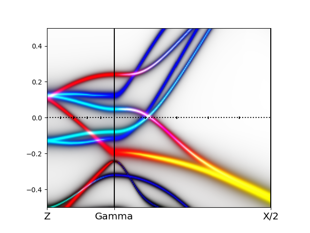
To orbitally resolve the spectra, we use dmftgk tool, already
described in FeSe tutorial.
At this stage, it is important to print projector into a single file
"Udmft.0", which can be achieved when mpi parallelization is switched
off. We hence eliminate "mpi_prefix.dat" and print the projector by
executing
x_dmft.py dmftu -g --band
Next we prepare a file dmftgke.in, which should look like:
e                    # mode [g/e]: we use mode to compute eigenvalues and eigenvectors
BasicArrays.dat      # filename for projector
0                    # matsubara
Ta2NiSe5O.energy     # LDA-energy-file, case.energy(so)(updn)
Ta2NiSe5O.klist_band # k-list
Ta2NiSe5O.rotlm      # for reciprocal vectors
Udmft.0              # filename for projector
0.0025               # gamma for non-correlated
0.0025               # gammac
sig.inp1_band  sig.inp2_band sig.inp3_band sig.inp4_band sig.inp5_band sig.inp6_band # self-energy filenames
eigenvalues.dat     # eigenvalues
UR.dat_             # right eigenvector in orbital basis
UL.dat_             # left eigenvector in orbital basis
-1.                 # emin for printed eigenvalues
 1.                 # emax for printed eigenvalues
if __name__ == '__main__':
    aspect_scale=1.0
    ....
    ....
    COHERENCE=True
    orb_plot=[0,1,3,3,3,3,3,3,3,3,2,3,3,3,3]  # should have integers 0,1,2 for red,green,blue
python wakplot_sophisticated.py eigenvalues.dat
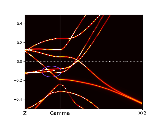
Next we repeat the same procedure for the low-temperature monoclinic
phase, which reveals a small semiconducting gap.
 We can convince
ourselves that it is semiconducting gap by looking into the
self-energy file sig.inp, which shows very small scattering
rate for all orbitals.
The orbitally resolved spectra of the monoclinic phase than looks like
We can convince
ourselves that it is semiconducting gap by looking into the
self-energy file sig.inp, which shows very small scattering
rate for all orbitals.
The orbitally resolved spectra of the monoclinic phase than looks like
 which has an unusual type of shape, and lead some to argue that bands
are formed by excitonic condensation.
which has an unusual type of shape, and lead some to argue that bands
are formed by excitonic condensation.
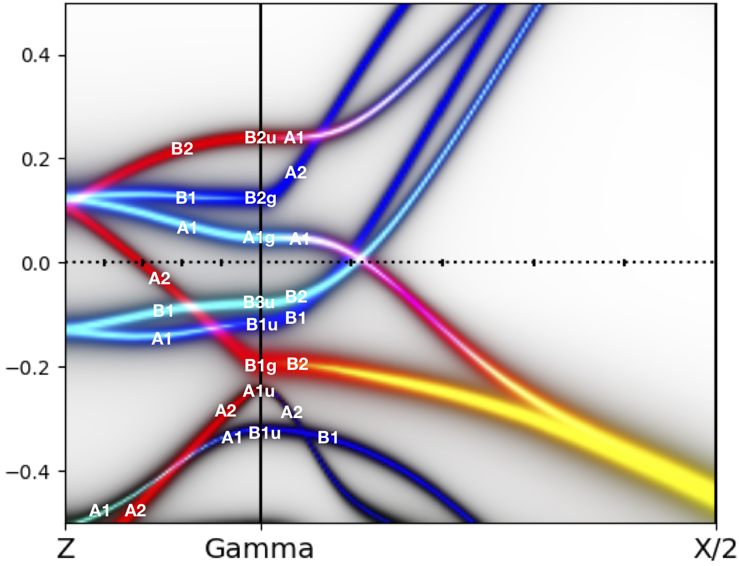
Finding the irreducible representation of the quasiparticle bands
The spectra which is very sharp has well defined quasiparticles, which
can be assigned irreducible representation, just like in the
band-theory case. We will use wien2k irrep tool to do
that. This tool needs a vector file, which contains quasiparticle
bands. To obtain such bands, we will run dmftp tool with the
following command
x_dmft.py dmftp --hermitianw
To see the quasiparticle-bands, which
will be analized by irrep, we need to display energies from
Ta2NiSe5M.outputdmfp. We could use wien2k tool spaghetti for
that purpose, but it is a bit tedious to substitute
Ta2NiSe5M.output1 by Ta2NiSe5M. outputdmfp, and also
resulting data is hard to analize in poscript form. We therefore use
alternative tool with similar capability
x_spaght.py. We will execute:
x_spaght.py Ta2NiSe5M.outputdmfp -y-0.5:0.5 -x: -g -Ry
 We choose to plot the bands in Ry units (-Ry) rather than eV, because it
will be easier to compare with data in case.outputir.
We also choose empty x-axis (-x:), which adds integer labels to each
k-point, which will be convenient in analyzing case.outputir.
We also show the grid (-g). This plot is
convenient to find which k-point is being analized by
irrep. Note that the mouse will show energy and momentum index of each
point.
We choose to plot the bands in Ry units (-Ry) rather than eV, because it
will be easier to compare with data in case.outputir.
We also choose empty x-axis (-x:), which adds integer labels to each
k-point, which will be convenient in analyzing case.outputir.
We also show the grid (-g). This plot is
convenient to find which k-point is being analized by
irrep. Note that the mouse will show energy and momentum index of each
point.
Next we produce irrep.def file for our analisys of dmft-vector file:
This produces irrep.def. We now need to replace Ta2NiSe5M.vector with
Ta2NiSe5M.vector_dmft in irrep.def file, i.e, irrep def
should have a line:
10,'./Ta2NiSe5M.vector_dmft', 'old', 'unformatted',9000
$WIENROOT/SRC_irrep/irrep irrep.def
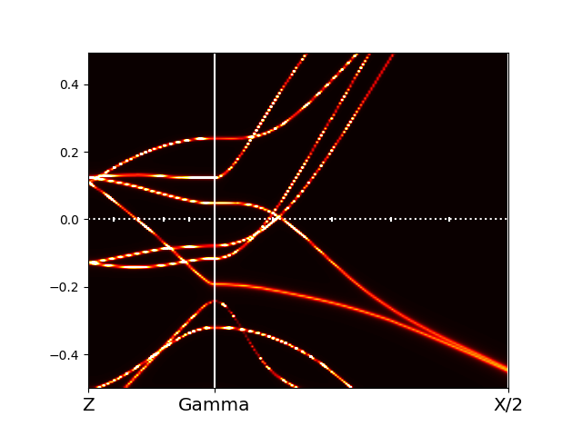
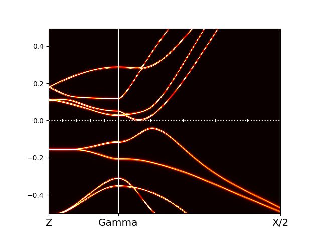
 We than repeat the same procedure for orhorombic phase, and the
quasiparticle plot is
We than repeat the same procedure for orhorombic phase, and the
quasiparticle plot is
 while the annotated spectral function is:
Plotting the Fermi surface of the orthorombic phase
To plot the Fermi surface, we will create another directory named FS,
and while in that directory we will copy crucial files from previous
real-axis work, i.e.,
dmft_copy.py ../onreal/
cp  ../onreal/SOlapm.dat .
x lapw0 -f Ta2NiSe5O
x_dmft.py lapw1
Next we construct self-energy with a single frequency in
sig.inp file, namely the zero frequency. We eliminate all other frequencies.
We than run dmft0 tool, which produces energies for all
k-points. We can either execute
or in metallic phase we can also assume that at the Fermi level the
scattering rate vanishes, therefore the eigenproblem is hermitian
x_dmft.py dmft0 --hermitian
xcrysden --bxsf Ta2NiSe5O.bxsf
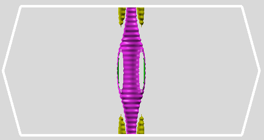
Constructing the cluster: Ti-Ni-Ti trimer
In the monoclinic phase, the chains of Ta atoms move parallel to the
chain direction, as shown below with orange arrows. As a result,
Ni-Ta distances, which were all equal in orthorombic phase,
disproportionate and hence each Ni atom comes closer with two Ta
octahedra (red arrows), while the other two octahedra move away (navy
blue arrows). As a result,
we have a trimer formation, indicated by red arrows in the figure.
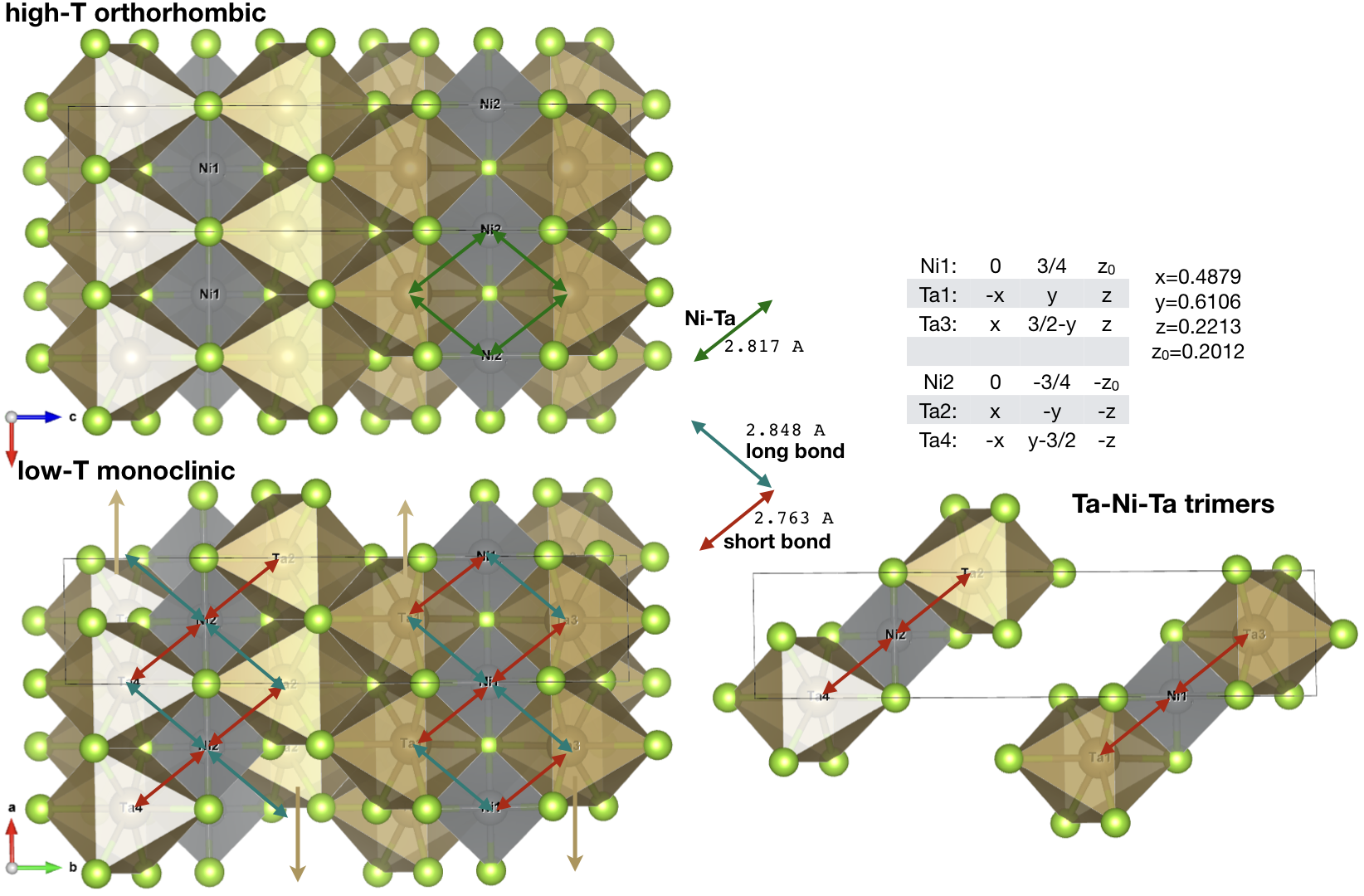 There are two non-overlaping trimes in the unit cell, with positions
specified in the above figure. We notice that Ni1 from structure file
forms bond with Ta1 and Ta3, while Ni2 forms bond with Ta2 and Ta4.
The positions of Ni1, Ta1, and Ta3 from the structure file are
(0,3/4,z0), (1-x,y,z), and (x,3/2-y,z). However, it turns out
that in the calculation a different set of atoms is actually
used. Even more confusing is the fact that positions of the atoms used
in the calculation depends on the order of the symmetry operations
specified in the structure file. If we reorder the symmetry
operations, we will be using a different (but equivalent) set of atoms
in the actual calculations. Within local approximations, this is not an
issue, however, for cluster constructions the bond between
Ni1:Ta(1-x,y,z)
is not the same as the bond between Ni1:Ta(-x,y,z). Hence, we need to
carefully select correct atoms which form clusters.
There are two non-overlaping trimes in the unit cell, with positions
specified in the above figure. We notice that Ni1 from structure file
forms bond with Ta1 and Ta3, while Ni2 forms bond with Ta2 and Ta4.
The positions of Ni1, Ta1, and Ta3 from the structure file are
(0,3/4,z0), (1-x,y,z), and (x,3/2-y,z). However, it turns out
that in the calculation a different set of atoms is actually
used. Even more confusing is the fact that positions of the atoms used
in the calculation depends on the order of the symmetry operations
specified in the structure file. If we reorder the symmetry
operations, we will be using a different (but equivalent) set of atoms
in the actual calculations. Within local approximations, this is not an
issue, however, for cluster constructions the bond between
Ni1:Ta(1-x,y,z)
is not the same as the bond between Ni1:Ta(-x,y,z). Hence, we need to
carefully select correct atoms which form clusters.
The file Ta2NiSe5M.outputdmf1 prints the actual positions of
atoms, as used in the calculations. The positions are:
Actual position of atom  1 is:  0.000000    0.750000    0.201210
Actual position of atom  2 is:  0.000000   -0.750000   -0.201210
Actual position of atom  3 is:  0.512048    0.610655    0.221366
Actual position of atom  4 is: -0.512048   -0.610655   -0.221366
Actual position of atom  5 is: -0.512048   -0.110655    0.221366
Actual position of atom  6 is:  0.512048    1.110655   -0.221366
Next we will modify Ta2NiSe5M.indmfl file, so that it will
correspond to the cluster (cellular-DMFT type) calculation. We create
a new directory, say nlHF, and copy previous real-axis data
into this directory by
To indicate that a set of atoms form a cluster in real space, we must
give all such atom the same index cix in the
Ta2NiSe5M.indmfl file. Each atom contains a line like
where the last number specifies cix. Notice that currently every atom
has its own cix-index, i.e.,
  2   2   1                           # L, qsplit, cix for Ni1
  2   2   2                           # L, qsplit, cix for Ni2
  2   2   3                           # L, qsplit, cix for Ta1
  2   2   4                           # L, qsplit, cix for Ta2
  2   2   5                           # L, qsplit, cix for Ta3
  2   2   6                           # L, qsplit, cix for Ta4
  2   2   1                           # L, qsplit, cix for Ni1
  2   2   2                           # L, qsplit, cix for Ni2
  2   2   1                           # L, qsplit, cix for Ta1
  2   2   2                           # L, qsplit, cix for Ta2
  2   2   1                           # L, qsplit, cix for Ta3
  2   2   2                           # L, qsplit, cix for Ta4
Next we want to take care of the necessary shifts of atoms. Currently,
we are specifying local rotation for each atom, but now we will
require also shift, in addition to rotation. For that, we will change
locrot, which is currently -1 (indicating nontrivial local rotation)
to -4. [ Notice that if local rotation was not necessary, we could use
flag -3, and omit local rotation. ] When locrot is -4 it means that
we will specify below 3x3 rotation as well as shift of an atom.
For example, for Ta(1), which currently contains this block
3     1  -1                           # iatom, nL, locrot
  2   2   3                           # L, qsplit, cix
-0.70889896 -0.28456479  0.64535660   # new x-axis
 0.70529973 -0.29095784  0.64644862   # new y-axis
 0.00381505  0.91343659  0.40696318   # new z-axis
3     1  -4                           # iatom, nL, locrot
  2   2   1                           # L, qsplit, cix
-0.70889896 -0.28456479  0.64535660   # new x-axis
 0.70529973 -0.29095784  0.64644862   # new y-axis
 0.00381505  0.91343659  0.40696318   # new z-axis
-1 0 0
We now repeat this procedure for all atoms. The resulting hader of the
Ta2NiSe5M.indmfl file will look like
111 198 1 5                           # hybridization band index nemin and nemax, renormalize for interstitials, $
0 0.025 0.025 200 -0.500000 0.500000  # matsubara, broadening-corr, broadening-noncorr, nomega, omega_min, omega_$
6                                     # number of correlated atoms
1     1  -1                           # iatom, nL, locrot
  2   2   1                           # L, qsplit, cix
-0.71715269 -0.69691608  0.00000000   # new x-axis
-0.69691608  0.71715269  0.00000000   # new y-axis
 0.00000000  0.00000000 -1.00000000   # new z-axis
2     1  -1                           # iatom, nL, locrot
  2   2   2                           # L, qsplit, cix
-0.71715269 -0.69691608  0.00000000   # new x-axis
-0.69691608  0.71715269  0.00000000   # new y-axis
 0.00000000  0.00000000 -1.00000000   # new z-axis
3     1  -4                           # iatom, nL, locrot
  2   2   1                           # L, qsplit, cix
-0.70889896 -0.28456479  0.64535660   # new x-axis
 0.70529973 -0.29095784  0.64644862   # new y-axis
 0.00381505  0.91343659  0.40696318   # new z-axis
-1 0 0
4     1  -4                           # iatom, nL, locrot
  2   2   2                           # L, qsplit, cix
-0.70889896 -0.28456479  0.64535660   # new x-axis
 0.70529973 -0.29095784  0.64644862   # new y-axis
 0.00381505  0.91343659  0.40696318   # new z-axis
1 0 0
5     1  -4                           # iatom, nL, locrot
  2   2   1                           # L, qsplit, cix
-0.70889896 -0.28456479  0.64535660   # new x-axis
 0.70529973 -0.29095784  0.64644862   # new y-axis
 0.00381505  0.91343659  0.40696318   # new z-axis
1 1 0
6     1  -4                           # iatom, nL, locrot
  2   2   2                           # L, qsplit, cix
-0.70889896 -0.28456479  0.64535660   # new x-axis
 0.70529973 -0.29095784  0.64644862   # new y-axis
 0.00381505  0.91343659  0.40696318   # new z-axis
-1 -2 0
The next lines specifies the number of cix-blocks and maximum
dimension, which used to be
#================ # Siginds and crystal-field transformations for correlated orbitals ================
6     5   5       # Number of independent kcix blocks, max dimension, max num-independent-components
1     5   5       # cix-num, dimension, num-independent-components
#================ # Siginds and crystal-field transformations for correlated orbitals ================
2    15  12       # Number of independent kcix blocks, max dimension, max num-independent-components
1    15  12       # cix-num, dimension, num-independent-components
Next we need to specify the order of the orbitals (their names), the
Sigind block, and the orbital
Transformation.
Lets just add Ni:d orbitals first, followed by Ta1, and Ta3 orbitals.
Sigind is than just a combination of Ni and Ta1+Ta3 components.
#---------------- # Independent components are --------------
'Ni(xz+yz)' 'Ni(xy)' 'Ni(xz-yz)' 'Ni(z^2)' 'Ni(x^2-y^2)' 'Ta1(xy)' 'Ta1(xz+yz)' 'Ta1(xz-yz)' 'Ta1(z^2)' 'Ta1(x^2-y^2)' 'Ta2(xy)' 'Ta2(xz+yz)' 'Ta2(xz-yz)' 'Ta2(z^2)' 'Ta2(x^2-y^2)'
#---------------- # Sigind follows --------------------------
 1  0  0  0  0 -11 0  0  0  0 -12 0  0  0  0
 0  2  0  0  0  0  0  0  0  0  0  0  0  0  0
 0  0  3  0  0  0  0  0  0  0  0  0  0  0  0
 0  0  0  4  0  0  0  0  0  0  0  0  0  0  0
 0  0  0  0  5  0  0  0  0  0  0  0  0  0  0
-11 0  0  0  0  6  0  0  0  0  0  0  0  0  0
 0  0  0  0  0  0  7  0  0  0  0  0  0  0  0
 0  0  0  0  0  0  0  8  0  0  0  0  0  0  0
 0  0  0  0  0  0  0  0  9  0  0  0  0  0  0
 0  0  0  0  0  0  0  0  0 10  0  0  0  0  0
-12 0  0  0  0  0  0  0  0  0  6  0  0  0  0
 0  0  0  0  0  0  0  0  0  0  0  7  0  0  0
 0  0  0  0  0  0  0  0  0  0  0  0  8  0  0
 0  0  0  0  0  0  0  0  0  0  0  0  0  9  0
 0  0  0  0  0  0  0  0  0  0  0  0  0  0 10
We could use positive numbers (11 and 12) for these off-diagonal
components. However, we than must add four more columns into the
self-energy (sig.inp) file, i.e., two new components of the
self-energy with real and imaginary part. If, however, a component
has a negative index, it means that it is frequency independent, and
just needs to be specified at the top of sig.inp file by
modifying s_oo, which is the self-energy at infinity. In this
case, the dynamic part of the self-energy does not need any extra
columns.
This is convenient when additing Hartree-Fock off-diagonal
self-energy, which is static.
Finally, the Transformation needs to reflect the chosen order of the
orbitals, i.e.,
 0.00000000  0.00000000    0.54510879  0.45039586    0.00000000  0.00000000   -0.54510879  0.45039586    0.00000000  0.00000000   0 0 0 0 0 0 0 0 0 0  0 0 0 0 0 0 0 0 0 0
-0.00402422 -0.65017840    0.00000000  0.00000000    0.39306964  0.00000000    0.00000000  0.00000000   -0.00402422  0.65017840   0 0 0 0 0 0 0 0 0 0  0 0 0 0 0 0 0 0 0 0
 0.00000000  0.00000000    0.45039586 -0.54510879    0.00000000  0.00000000   -0.45039586 -0.54510879    0.00000000  0.00000000   0 0 0 0 0 0 0 0 0 0  0 0 0 0 0 0 0 0 0 0
 0.07091418  0.27617429    0.00000000  0.00000000    0.91509447  0.00000000    0.00000000  0.00000000    0.07091418 -0.27617429   0 0 0 0 0 0 0 0 0 0  0 0 0 0 0 0 0 0 0 0
 0.70353038 -0.03155676    0.00000000  0.00000000   -0.08999096  0.00000000    0.00000000  0.00000000    0.70353038  0.03155676   0 0 0 0 0 0 0 0 0 0  0 0 0 0 0 0 0 0 0 0
 0 0 0 0 0 0 0 0 0 0 -0.00489259 -0.69416147    0.13411482 -0.00335834    0.01535367  0.00000000   -0.13411482 -0.00335834   -0.00489259  0.69416147   0 0 0 0 0 0 0 0 0 0
 0 0 0 0 0 0 0 0 0 0 -0.01110550  0.08356195    0.43666523  0.53858106    0.15587173  0.00000000   -0.43666523  0.53858106   -0.01110550 -0.08356195   0 0 0 0 0 0 0 0 0 0
 0 0 0 0 0 0 0 0 0 0 -0.10146142  0.10139414    0.49645295 -0.45391163    0.23204965  0.00000000   -0.49645295 -0.45391163   -0.10146142 -0.10139414   0 0 0 0 0 0 0 0 0 0
 0 0 0 0 0 0 0 0 0 0  0.07153571 -0.02612921   -0.18700502  0.01851820    0.95800429  0.00000000    0.18700502  0.01851820    0.07153571  0.02612921   0 0 0 0 0 0 0 0 0 0
 0 0 0 0 0 0 0 0 0 0  0.69601793  0.01391990    0.09950018 -0.05950198   -0.06204045  0.00000000   -0.09950018 -0.05950198    0.69601793 -0.01391990   0 0 0 0 0 0 0 0 0 0
 0 0 0 0 0 0 0 0 0 0  0 0 0 0 0 0 0 0 0 0   -0.00489259 -0.69416147    0.13411482 -0.00335834    0.01535367  0.00000000   -0.13411482 -0.00335834   -0.00489259  0.69416147
 0 0 0 0 0 0 0 0 0 0  0 0 0 0 0 0 0 0 0 0   -0.01110550  0.08356195    0.43666523  0.53858106    0.15587173  0.00000000   -0.43666523  0.53858106   -0.01110550 -0.08356195
 0 0 0 0 0 0 0 0 0 0  0 0 0 0 0 0 0 0 0 0   -0.10146142  0.10139414    0.49645295 -0.45391163    0.23204965  0.00000000   -0.49645295 -0.45391163   -0.10146142 -0.10139414
 0 0 0 0 0 0 0 0 0 0  0 0 0 0 0 0 0 0 0 0    0.07153571 -0.02612921   -0.18700502  0.01851820    0.95800429  0.00000000    0.18700502  0.01851820    0.07153571  0.02612921
 0 0 0 0 0 0 0 0 0 0  0 0 0 0 0 0 0 0 0 0    0.69601793  0.01391990    0.09950018 -0.05950198   -0.06204045  0.00000000   -0.09950018 -0.05950198    0.69601793 -0.01391990
2 15 12 # cix-num, dimension, num-independent-components
# s_oo= [58.34111987610038, 57.99864526007574, 58.66792046452633, 58.15374868968896, 58.68284274853787, 11.52900772267362, 11.456232499198762, 11.35548455310819, 11.192604230189128, 11.111987546730667]
# Edc= [59.842921188735275, 59.83356456338613, 59.79961530249243, 59.79826650028635, 59.826546613721476, 8.319863999593021, 8.299004410493579, 8.302522649084414, 8.236828534352366, 8.22545468607832]
# s_oo= [58.34111987610038, 57.99864526007574, 58.66792046452633, 58.15374868968896, 58.68284274853787, 11.52900772267362, 11.456232499198762, 11.35548455310819, 11.192604230189128, 11.111987546730667, 0, 0]
# Edc= [59.842921188735275, 59.83356456338613, 59.79961530249243, 59.79826650028635, 59.826546613721476, 8.319863999593021, 8.299004410493579, 8.302522649084414, 8.236828534352366, 8.22545468607832, 0, 0]
To check that Ta2NiSe5M.indmfl was properly modified, we will
plot density of states, and compare with previous results. Since the
off-diagonal self-energy is set to zero here, the results
for density of states and all green's functions should be
identical. Notice however, that the hybridizations can be very
different, because the hybridization contains the inverse of the green's
function, which is now a much larger (15x15) matrix. The hybridization
now correponds to the cluster-DMFT hybridization for the trimer.
x lapw0 -f Ta2NiSe5M
x_dmft.py lapw1
x_dmft.py dmft1
The local green's function from previous real-axis run and this one
should match, which means that columns 1 to 11 of previous
../onreal/Ta2NiSe5M.gc1 and current Ta2NiSe5M.gc1 should
match. In addition, the columns of 12 to 21 of Ta2NiSe5M.gc1
should match columns 2 to 11 of previous
../onreal/Ta2NiSe5M.gc3. For example, a plot of
plot -g -u1:3,1:13 -x-3:3 Ta2NiSe5M.gc1 -u1:3 ../onreal/Ta2NiSe5M.gc1 ../onreal/Ta2NiSe5M.gc1
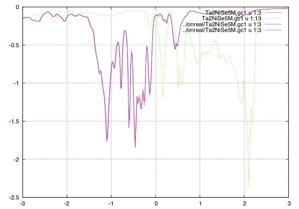
We also need to check the symmetry of the off-diagonal green's
function by displaying 23-th and 25-th column (11-th and 12-th
component of the off-diagonal green's function).
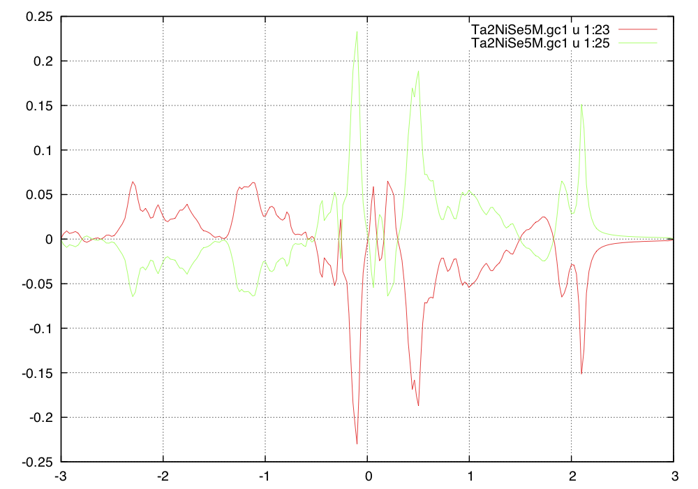 We notice that in this monoclinic phase, the symmetry requires Ni-Ta1
Green's function to have opposite sign to Ni-Ta2 bond. We could add an extra pi
phase to the Ta2 orbitals, and than the two components would be
identical. We note that the self-energy and the Green's function have
the same symmetry, hence if we redefine the Ta2 orbitals with opposite
sign, we would need only
11 component self-energy rather than
12 component. But we will not do that now.
We notice that in this monoclinic phase, the symmetry requires Ni-Ta1
Green's function to have opposite sign to Ni-Ta2 bond. We could add an extra pi
phase to the Ta2 orbitals, and than the two components would be
identical. We note that the self-energy and the Green's function have
the same symmetry, hence if we redefine the Ta2 orbitals with opposite
sign, we would need only
11 component self-energy rather than
12 component. But we will not do that now.
Non-local Hartree-Fock
Now that we have the trimer cluster, we can perform Hartree-Fock
calculation for the non-local components. In particular, we can
consider the effects on non-local components of the screened Coulomb
repulsion, i.e.,
 .
.
The Hartree part of the Coulomb interaction has been already correctly taken into
account by LDA/GGA, hence we should not double-count the
Hartree-part. However, the exchange and correlation between sites is completely
missing in LDA/GGA or DMFT, hence at the lowest order, we need to
consider the exchange contribution of the form

To consider the self-energy between Ni(xz+yz) and Ta(xy) orbital, we
thus need the corresponding entry in the density matrix. We will thus
run dmft1 on imaginary axis, and check the density matrix in
Ta2NiSe5M.outdmft1.
We first save the real axis self-energy and replace it with the
imaginary axis self-energy.
mv sig.inp sig.inp_real_axis
cp ../sig.inp .
We than add two more components to the header of the self-energy, just
like before, i.e., the existing header
# s_oo= [58.33960607278515, 57.99799075799591, 58.66764718991543, 58.1528394846167, 58.68155194019003, 11.52723220068357, 11.45504198755027, 11.35418395795326, 11.19128337408098, 11.11088607272979]
# Edc= [59.841935471914276, 59.83260781272945, 59.79850099666909, 59.79715237803764, 59.82554966046209, 8.318434113332705, 8.297724288472981, 8.301180281321397, 8.23549025137547, 8.224172638351167]
is replaced by
# s_oo= [58.33960607278515, 57.99799075799591, 58.66764718991543, 58.1528394846167, 58.68155194019003, 11.52723220068357, 11.45504198755027, 11.35418395795326, 11.19128337408098, 11.11088607272979, 0, 0]
# Edc= [59.841935471914276, 59.83260781272945, 59.79850099666909, 59.79715237803764, 59.82554966046209, 8.318434113332705, 8.297724288472981, 8.301180281321397, 8.23549025137547, 8.224172638351167, 0, 0]
We change the flag matsubara to 1 in Ta2NiSe5M.indmfl to
perform calculation on imaginary axis. And than we run
Than we look into Ta2NiSe5M.outdmft1 how the density matrix
looks like
:NCOR   12.994665  1   15  # nf, icix, cixdm
   1.7166866   -0.0000000     -0.0000755   -0.0000000     -0.0040139   -0.0000000     -0.0000393   -0.0000000     -0.0000129    0.0000000     -0.0275268   -0.0000000     -0.0872614    0.0000000     -0.0468143   -0.0000000      0.0544655   -0.0000000     -0.0224366
  -0.0000755    0.0000000      1.8119760    0.0000000      0.0000172   -0.0000000     -0.0039443   -0.0000000     -0.0048936   -0.0000000      0.0955963    0.0000000      0.0540922    0.0000000     -0.0030930    0.0000000      0.0239057   -0.0000000     -0.0313942
  -0.0040139    0.0000000      0.0000172    0.0000000      1.6023202    0.0000000      0.0000040   -0.0000000     -0.0000009    0.0000000     -0.0500300    0.0000000      0.0658608   -0.0000000      0.1551905   -0.0000000     -0.0459625   -0.0000000     -0.0036675
  -0.0000393    0.0000000     -0.0039443    0.0000000      0.0000040    0.0000000      1.7505693    0.0000000     -0.0135653    0.0000000      0.0110898   -0.0000000      0.0319096    0.0000000      0.1413475   -0.0000000     -0.0643905   -0.0000000      0.0137550
  -0.0000129   -0.0000000     -0.0048936    0.0000000     -0.0000009   -0.0000000     -0.0135653   -0.0000000      1.6309636   -0.0000000     -0.0067397   -0.0000000     -0.1657144    0.0000000     -0.1909387   -0.0000000      0.1093709    0.0000000      0.0035428
  -0.0275268    0.0000000      0.0955963   -0.0000000     -0.0500300   -0.0000000      0.0110898    0.0000000     -0.0067397    0.0000000      0.3507117   -0.0000000     -0.0196900    0.0000000      0.0080640   -0.0000000      0.0266478    0.0000000      0.0007574
  -0.0872614   -0.0000000      0.0540922   -0.0000000      0.0658608    0.0000000      0.0319096   -0.0000000     -0.1657144   -0.0000000     -0.0196900   -0.0000000      0.3827676    0.0000000      0.0096011    0.0000000     -0.0031817   -0.0000000      0.0021048
  -0.0468143    0.0000000     -0.0030930   -0.0000000      0.1551905    0.0000000      0.1413475    0.0000000     -0.1909387    0.0000000      0.0080640    0.0000000      0.0096011   -0.0000000      0.4679031   -0.0000000     -0.0091721    0.0000000      0.0022629
   0.0544655    0.0000000      0.0239057    0.0000000     -0.0459625    0.0000000     -0.0643905    0.0000000      0.1093709   -0.0000000      0.0266478   -0.0000000     -0.0031817    0.0000000     -0.0091721   -0.0000000      0.4997402    0.0000000     -0.0008033
  -0.0224366    0.0000000     -0.0313942    0.0000000     -0.0036675    0.0000000      0.0137550    0.0000000      0.0035428   -0.0000000      0.0007574    0.0000000      0.0021048   -0.0000000      0.0022629   -0.0000000     -0.0008033   -0.0000000      0.5399797
   0.0275940   -0.0000000      0.0955899   -0.0000000      0.0500146    0.0000000      0.0110912   -0.0000000     -0.0067380    0.0000000      0.0042034   -0.0000000      0.0000261    0.0000000      0.0104573    0.0000000      0.0070014   -0.0000000     -0.0085243
   0.0872932   -0.0000000      0.0540954   -0.0000000     -0.0658473   -0.0000000      0.0319100   -0.0000000     -0.1657210   -0.0000000     -0.0000452   -0.0000000     -0.0051224    0.0000000     -0.0226664   -0.0000000      0.0233843    0.0000000     -0.0035038
   0.0468201    0.0000000     -0.0031192   -0.0000000     -0.1551889   -0.0000000      0.1413369    0.0000000     -0.1909445   -0.0000000      0.0104435   -0.0000000     -0.0226546   -0.0000000     -0.0497412   -0.0000000      0.0170714    0.0000000      0.0019080
  -0.0544860   -0.0000000      0.0239183    0.0000000      0.0459665   -0.0000000     -0.0643833   -0.0000000      0.1093756    0.0000000      0.0069854    0.0000000      0.0233694   -0.0000000      0.0170699    0.0000000     -0.0061118   -0.0000000     -0.0023756
   0.0224315    0.0000000     -0.0314047   -0.0000000      0.0036647    0.0000000      0.0137501   -0.0000000      0.0035420    0.0000000     -0.0085373   -0.0000000     -0.0034940   -0.0000000      0.0019112    0.0000000     -0.0023789    0.0000000      0.0010117
We notice that all off-diagonal components are pretty small, and hence
in the high-temperature phase the corrections to the band structure
due to screened non-local contribution is small. However, in the
symmetry broken phase, some components which are not allowed in the
orthorombic phase, can become nonzero. The non-local
Ni(xz+yz):Ta(xy), which is finite only within our chosen trimer,
(non-zero on red bonds in the figure, and vanishes on the blue)
breaks the symmetry of the high-temperature phase, and is thus not
allowed in the orthorombic phase. But is allowed in the monoclinic
phase. We will thus set it to some nonzero-value, and optimize it
self-consistently for choosen value of non-local Coulomb interaction
V. Let's consider V=3eV, which is half of the on-site interaction on
Ta. We will set self-energy first to a value 0.35eV, i.e., header of
the sig.inp becomes
# s_oo= [58.33960607278515, 57.99799075799591, 58.66764718991543, 58.1528394846167, 58.68155194019003, 11.52723220068357, 11.45504198755027, 11.35418395795326, 11.19128337408098, 11.11088607272979, -0.35,0.35]
# Edc= [59.841935471914276, 59.83260781272945, 59.79850099666909, 59.79715237803764, 59.82554966046209, 8.318434113332705, 8.297724288472981, 8.301180281321397, 8.23549025137547, 8.224172638351167, 0.0, 0.0]
and we will rerun
:NCOR   12.985283  1   15  # nf, icix, cixdm
   1.7063583   -0.0000000     -0.0000687    0.0000000      0.0235177   -0.0000000     -0.0000345    0.0000000     -0.0000082    0.0000000      0.1168346   -0.0000000     -0.0826159    0.0000000     -0.0411286   -0.0000000      0.0539939   -0.0000000     -0.0210488
  -0.0000687   -0.0000000      1.8050129    0.0000000      0.0000301   -0.0000000     -0.0021135   -0.0000000     -0.0051496    0.0000000      0.0973357    0.0000000      0.0557467    0.0000000     -0.0075498   -0.0000000      0.0233133    0.0000000     -0.0325156
   0.0235177    0.0000000      0.0000301    0.0000000      1.6058929    0.0000000      0.0000002   -0.0000000      0.0000003    0.0000000     -0.0455411    0.0000000      0.0676536    0.0000000      0.1479968   -0.0000000     -0.0424905   -0.0000000     -0.0063524
  -0.0000345   -0.0000000     -0.0021135    0.0000000      0.0000002    0.0000000      1.7506449    0.0000000     -0.0135649   -0.0000000      0.0113038    0.0000000      0.0312383    0.0000000      0.1421482   -0.0000000     -0.0638839    0.0000000      0.0138251
  -0.0000082   -0.0000000     -0.0051496   -0.0000000      0.0000003   -0.0000000     -0.0135649    0.0000000      1.6311759    0.0000000     -0.0069271   -0.0000000     -0.1662423    0.0000000     -0.1908940   -0.0000000      0.1094664    0.0000000      0.0033805
   0.1168346    0.0000000      0.0973357   -0.0000000     -0.0455411   -0.0000000      0.0113038   -0.0000000     -0.0069271    0.0000000      0.3609223    0.0000000     -0.0230903    0.0000000     -0.0085177   -0.0000000      0.0382409    0.0000000     -0.0075248
  -0.0826159   -0.0000000      0.0557467   -0.0000000      0.0676536   -0.0000000      0.0312383   -0.0000000     -0.1662423   -0.0000000     -0.0230903   -0.0000000      0.3809779    0.0000000      0.0116748    0.0000000     -0.0009808   -0.0000000      0.0025175
  -0.0411286    0.0000000     -0.0075498    0.0000000      0.1479968    0.0000000      0.1421482    0.0000000     -0.1908940    0.0000000     -0.0085177    0.0000000      0.0116748   -0.0000000      0.4621919   -0.0000000     -0.0110672    0.0000000      0.0006904
   0.0539939    0.0000000      0.0233133   -0.0000000     -0.0424905    0.0000000     -0.0638839   -0.0000000      0.1094664   -0.0000000      0.0382409   -0.0000000     -0.0009808    0.0000000     -0.0110672   -0.0000000      0.4997230    0.0000000     -0.0016861
  -0.0210488    0.0000000     -0.0325156   -0.0000000     -0.0063524    0.0000000      0.0138251    0.0000000      0.0033805    0.0000000     -0.0075248    0.0000000      0.0025175   -0.0000000      0.0006904   -0.0000000     -0.0016861   -0.0000000      0.5391607
  -0.1167733   -0.0000000      0.0972739    0.0000000      0.0454683   -0.0000000      0.0113219    0.0000000     -0.0069194   -0.0000000     -0.0116659   -0.0000000      0.0046546    0.0000000      0.0255121    0.0000000     -0.0044614   -0.0000000     -0.0014033
   0.0826389   -0.0000000      0.0557496   -0.0000000     -0.0676305   -0.0000000      0.0312384   -0.0000000     -0.1662507   -0.0000000      0.0046007   -0.0000000     -0.0043375    0.0000000     -0.0221338    0.0000000      0.0214008   -0.0000000     -0.0034290
   0.0411290   -0.0000000     -0.0075684    0.0000000     -0.1479888   -0.0000000      0.1421394   -0.0000000     -0.1908945    0.0000000      0.0254995   -0.0000000     -0.0221219   -0.0000000     -0.0500560    0.0000000      0.0175730    0.0000000      0.0020463
  -0.0540128   -0.0000000      0.0233154    0.0000000      0.0424935    0.0000000     -0.0638766    0.0000000      0.1094696    0.0000000     -0.0044630    0.0000000      0.0213845    0.0000000      0.0175725    0.0000000     -0.0060172   -0.0000000     -0.0020753
   0.0210495   -0.0000000     -0.0325247   -0.0000000      0.0063521   -0.0000000      0.0138209   -0.0000000      0.0033808    0.0000000     -0.0014127   -0.0000000     -0.0034195    0.0000000      0.0020470   -0.0000000     -0.0020772    0.0000000      0.0010964
Now the corresponding density matrix entry at (1,6) and (1,11) as well
as at (6,1) and and (11,1), corresponding to Ni(xz+yz):Ta(xy), becomes
equal to 0.1168346. More precisely, the (1,6) and (6,1) component is
0.1168346, and (1,11) and (11,1) is -0.1168346. With V=3eV, this
requires self-energy of 0.35eV, i.e., our input value for the
self-energy.
We note that such non-local Coulomb interaction is finite, but rather
small, and the value of 3eV is somewhat too large to be
realistic. Consider the Coulomb repulsion on Ta atom, which we estimated to
be U=6eV and J=0.8eV. This translates to Yukawa screening of
lambda=0.408/rB, and dielectric screening epslion=1.260. This can be
simply obtained by running
RCoulombU.py -U 6. -J 0.8
V(r) = 2Ry \frac{\exp(-\lambda\,r)}{\epsilon\, r}
and a simplified estimation of the non-local Coulomb repulsion at
distance 5.22 bohr radius (corresponding to 2.76A trimer distance) is
0.5eV. Taking the value of U=8eV on Ni will make such non-local
repulsion even smaller. However, such non-local correlations can be
generated by purely local interaction, when considering higher order
processes, or equivalently, cluster-DMFT. We should thus consider such
non-local Hartree-Fock calculation as a qualitative estimation of the
non-local effects, which are currently hard to compute by the
available impurity solvers.
Now that we have required non-local self-energy, we switch back to
real axis, and plot the spectral function.
We first copy the saved self-energy
cp sig.inp_real_axis sig.inp
x_dmft.py lapw1 --band
x_dmft.py dmftp
We can now plot also the orbitally resolved spectra as above, using
dmftgk tool, which gives the following plot:
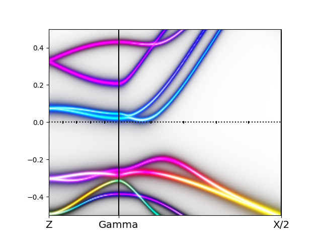
Structural optimization with and withouth non-local Hartree Fock self-energy
We can relax internal parameters of the monoclinic crystal structure
within eDMFT. It turns out that the monoclinic distortion is not
stable, and the internal structural parameters closely resemble those of the
high-temperature orthorhombic phase (even though the unit cell has
monoclinic distortion).
Now we can also check if the broaken symmetry, which we guessed above with
the non-local Hartee Fock, stabilizes the monoclinic phase. Note that
the symmetry of the Ta-Ni self-energy corresponds to B3g irrep, which is indeed experimentally
determined symmetry of the order parameter.
Indeed
this order parameter stabilizes the monoclinic phase, and the Ta-Ni
bonds disproportionate into long and short.
To do this type of calculation, we will create yet another directory relax,
and copy data from previous directory nlHF the input files
dmft_copy.py  ../nlHF/
cp ../nlHF/sig.inp_imag_axis sig.inp
We next edit Ta2NiSe5M.in2 file, and set TOT to FOR, i.e., the
first line now looks like
FOR (TOT,FOR,QTL,EFG,FERMI)
and we will also change the mixer to MSR1a, which mixes both the
charge density and atomic coordinates for relaxation of the
structure. The first line of the Ta2NiSe5M.inm will look like
MSR1a 0.0 YES (BROYD/PRATT, BG charge (-1 for core hole), norm)
At the moment the run will still fail because case.indmfi and
case.indmfl files are incompatible. We created cluster in
case.indmfl, but we did not appropriately update
case.indmfi.
We will edit case.indmfi such that it will contain only one
impurity problem (actually cluster problem now), and identical
Sigind matrix as found in case.indmfl.
Our new case.indmfi looks like:
1   # number of sigind blocks
15  # dimension of this sigind block
 1  0  0  0  0 -11 0  0  0  0 -12 0  0  0  0
 0  2  0  0  0  0  0  0  0  0  0  0  0  0  0
 0  0  3  0  0  0  0  0  0  0  0  0  0  0  0
 0  0  0  4  0  0  0  0  0  0  0  0  0  0  0
 0  0  0  0  5  0  0  0  0  0  0  0  0  0  0
-11 0  0  0  0  6  0  0  0  0  0  0  0  0  0
 0  0  0  0  0  0  7  0  0  0  0  0  0  0  0
 0  0  0  0  0  0  0  8  0  0  0  0  0  0  0
 0  0  0  0  0  0  0  0  9  0  0  0  0  0  0
 0  0  0  0  0  0  0  0  0 10  0  0  0  0  0
-12 0  0  0  0  0  0  0  0  0  6  0  0  0  0
 0  0  0  0  0  0  0  0  0  0  0  7  0  0  0
 0  0  0  0  0  0  0  0  0  0  0  0  8  0  0
 0  0  0  0  0  0  0  0  0  0  0  0  0  9  0
 0  0  0  0  0  0  0  0  0  0  0  0  0  0 10
We will add an option
into params.dat file, because we do not have cluster-DMFT
solver to compute self-consistent cluster self-energy. We will keep
the single-site self-energy + Hartree Fock value for now, and relax
structure by optimizing charge density. We note that the band gap in
this system is not opened by correlations, but it is a band gap, in which
the DMFT self-energy is quite insensitive to small changes of
the structural parameters, as seen by structural relaxation of the
single-site DMFT calculation.
Now we are ready to submit the job.
After a few hundred iterations, the forces are reduced below 0.3, with
converged charge, and relaxation confirms the
disproportionate bonds, namely, the two inequivalent Ta-Ni distances are
theory:
Ni-Ta1 = 2.759 Å
Ni-Ta2 = 2.871 Å
experiment:
Ni-Ta1 = 2.763 Å
Ni-Ta2 = 2.848 Å
theory:
Ni = [0,3/4,0.19482]
Ta = [0.51826406,0.60978623,0.21383811]
Se1= [1/2,3/4,0.32546859]
Se2= [0.00089185,0.55309075,0.36032579]
Se3= [0.00502183,0.64416589,0.06569934]
experiment:
Ni = [0,3/4,0.20121]
Ta = [0.512048,0.610655,0.221366]
Se1= [1/2,3/4,0.327557]
Se2= [0.991386,0.548924,0.354601]
Se3= [0.991752,0.638047,0.079931]
Optical conductivity
For optics calculation we create anothe directory optics and
copy the real-axis data into the new directory:
We will increase the k-mesh, as converged optics calculation needs
very fine mesh. For finite plot below, we will use 5000 k-points. But
when testing the input parameters, much smaller mesh should be first attempted.
x kgen -f Ta2NiSe5M
   5000,
x lapw0 -f Ta2NiSe5M
x_dmft.py lapw1
Next print projector, but first remove parallelization, because
projector should be stored in a single file:
rm mpi_prefix.dat
x_dmft.py dmftu
Next, prepare the input file for computing the optics matrix elements
within wien2k. The input files should be Ta2NiSe5M.inop:
99999 1       number of k-points, first k-point
-5.0 3.0 9999 Emin, Emax for matrix elements, NBvalMAX
2             number of choices (columns in *outmat): 2: hex or tetrag. case
1             Re xx
3             Re zz
ON            ON/OFF   writes MME to unit 4
Next run
x optic[c] [-so] [-up] -f Ta2NiSe5M
Next we prepare an input file for dmft-optics calculation
dmftopt.in, which should look like
    0          # Temperature  (this is new in 2014)
    Ta2NiSe5M  # case
    0.002      # gamma  -- broadening of all bands / we recommend to keep nonzero value
    0.0        # gammac -- broadening of the correlated bands (in addition to the self-energy)
    4.0        # ommax  -- maximum frequency for the optics calculation
    1e-2       # delta  -- minimum separation of frequency for logarithmic mesh in frequency
    50         # Nd     -- number of points in each linear mesh, a subset of logarithmic mesh
    T          # Qsym: [F|T]. Do we need to symmetrize? (over all k-points or just irreducible.) If Qsym is F, it goes over irreducible, if Qsym is T, it goes over all.
    F          # InterbandOnly [F|T] (F -- all, T--interband)
    5          # dwindow -- Not all bands are used in computation of optics, but only those from [-omeg-dwindow, omega+dwindow]. You should increase this to make sure you are not cutting some bands which are needed.
    3          # Ndirection -- How many optics type do you want to compute: xx, yy, zz,...
    1.0 0.0 0.0    # alphaV(1,:)
    0.0 0.0 0.0    # alphaV(2,:)
    0.0 0.0 0.0    # alphaV(3,:)
    0.0 0.0 0.0    # alphaV(1,:)
    0.0 1.0 0.0    # alphaV(2,:)
    0.0 0.0 0.0    # alphaV(3,:)
    0.0 0.0 0.0    # alphaV(1,:)
    0.0 0.0 0.0    # alphaV(2,:)
    0.0 0.0 1.0    # alphaV(3,:)
If temperature is not very high (like in the Earth's core) we can safely
set temperature to 0, and we will still get very accurate results,
corresponding to the temperature at which DMFT was run, because we have
scattering rate from DMFT calculations, which gives finite width to
the Drude peak. The temperature in optics calculation is just the
Fermi function temperature in calculating the bubble, and is
unfortunately quite expensive to use, i.e., the step function needs to
be replaced by dense mesh of points near the step, and for most cases
does not make noticable difference.
Here we choose very small broadening gamma=0.002, which will produce
very sharp features in the optical spectra, and requires very many k-points. In
most calculations, we could increase gamma for factor of 5, and reduce
number of k-points, and still resolve most of the features. We will
broaden the spectra at the end, with the tool broad, which has
very similar effect as increasing gamma. Note however, that we need
finite gamma to not loose weight in the integration over frequency,
which is done analytically.
The frequency mesh, which is used in the optics calculation for the
internal frequency integration, is a hybrid of
equidistant and logarithmic mesh, sketched in this figure:
 For very low frequency, where we expect Drude peak in metals, we
use very fine mesh, which starts with distance delta (here 1e-2). In
many metals at low-T one needs to reduce this parameter, to resolve
the Drude peak. Next, we use 2*Nd+1 (here 2*50+1=101) points in
equidistant mesh, to resolve every frequency between 0 and Nd*delta
with high accuracy. In the next step, we keep only every second point
of the previous mesh, and extent it to 2*Nd*delta, using again 2*Nd+1
points. We keep increasing the frequency intervals until we reach
ommax (here 4), which is reached when delta*Nd*2**N0==ommax. N0 here
determines number of levels at which we double the extent of the mesh.
The mesh with Nd=50 is very precise, and in many situations one could
use Nd=10 or Nd=5, and still get very reasonable optics spectra. We
suggest one to experiment with these parameters when number of
k-points is not too large, and cutoff frequency ommax is not too
large, and than increase number of k-points once a good set of
parameters is found.
For very low frequency, where we expect Drude peak in metals, we
use very fine mesh, which starts with distance delta (here 1e-2). In
many metals at low-T one needs to reduce this parameter, to resolve
the Drude peak. Next, we use 2*Nd+1 (here 2*50+1=101) points in
equidistant mesh, to resolve every frequency between 0 and Nd*delta
with high accuracy. In the next step, we keep only every second point
of the previous mesh, and extent it to 2*Nd*delta, using again 2*Nd+1
points. We keep increasing the frequency intervals until we reach
ommax (here 4), which is reached when delta*Nd*2**N0==ommax. N0 here
determines number of levels at which we double the extent of the mesh.
The mesh with Nd=50 is very precise, and in many situations one could
use Nd=10 or Nd=5, and still get very reasonable optics spectra. We
suggest one to experiment with these parameters when number of
k-points is not too large, and cutoff frequency ommax is not too
large, and than increase number of k-points once a good set of
parameters is found.
Qsym should be set to true whenever we need more than just the average
optical conductivity. Only for the average conductivity
(sigma_xx+sigma_yy+sigma_zz)/3. it is sufficient to consider the
irreducible k-points only.
While this symmetrization works quite well in most cases, we advice
one to check it in any particular low symmetry calculation, by using
calculation with all k-points in the first Brillouine zone (not just
irreducible) and seeting Qsym to F. The symmetrization is done in
similar way as in wien2k optics calculation.
InterbandOnly is normally set to F, because within DMFT it is hard to
split the interband contributions from Drude peak, and even though the
equation is straighforward, the result might be unexpected.
Finally, we can calculate several directions of optics
simultaneously. Here we choose three directions, sigmaxx,
sigmayy and sigmazz. Any other entry in the
matrix is possible, in principle, but has not been well tested.
Now we can remove large vector file, which is
hard to copy when submitting the job, and proceed only with the essential
files. The optics calculation needs the following files:
case.mommat2, case.symop, case.symmat,
case.energy[so][updn], sig.inp?,
Udmft.0, BasicArrays, and dmftopt.in.
We can run the executable dmftopt in parallel, for example
mpirun [-n nkp] dmftopt > nohup.dat
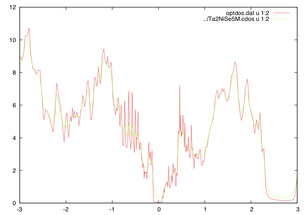 Notice that because we use here very small broadening, the gap is very
clearly developed, while in dmft1 the gap was somewhat less
well developed due to finite broadening.
Notice that because we use here very small broadening, the gap is very
clearly developed, while in dmft1 the gap was somewhat less
well developed due to finite broadening.
The calculated optical conductivity is found in optics.dat, and
should look like:
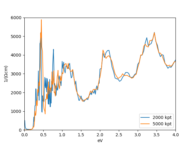 Notice that the calculation with 2000 k-points and 5000 k-points is
similar, newertheless the details of the peaks are somewhat different
in the two calculations. The 2000 k-point calculation seems to have s
small peak in the gap, which completely dissapears when using 5000 k-points.
Finally, it is advisable to broaden the sharp features from the
calculated optical conductivity, which has similar effect as
increasing gamma in the calculation, except that in postprocessing we
can apply broadening many times, until we find reasonably smooth curve. For
example, with gaussian convolution of width 0.02eV
Notice that the calculation with 2000 k-points and 5000 k-points is
similar, newertheless the details of the peaks are somewhat different
in the two calculations. The 2000 k-point calculation seems to have s
small peak in the gap, which completely dissapears when using 5000 k-points.
Finally, it is advisable to broaden the sharp features from the
calculated optical conductivity, which has similar effect as
increasing gamma in the calculation, except that in postprocessing we
can apply broadening many times, until we find reasonably smooth curve. For
example, with gaussian convolution of width 0.02eV
broad -w 0.02 optics.dat > b_optics.dat
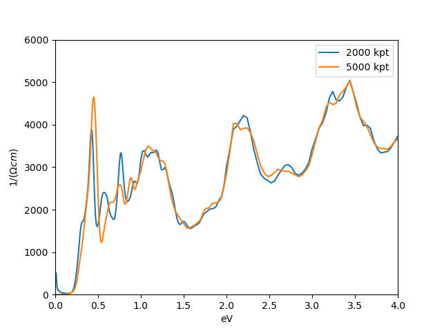 The first sharp peak is clearly much better developed at 5000 k-points
than with 2000 k-points. Finally, the other two directions have less low
energy features, and are easier to converge:
The first sharp peak is clearly much better developed at 5000 k-points
than with 2000 k-points. Finally, the other two directions have less low
energy features, and are easier to converge:
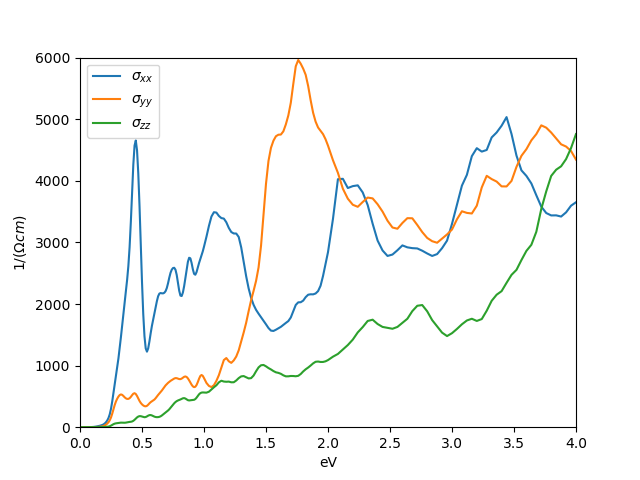 Comparison with experiment (from PRB 95, 195144 (2017)) reveals very
reasonable agreement of all three directions:
Comparison with experiment (from PRB 95, 195144 (2017)) reveals very
reasonable agreement of all three directions:
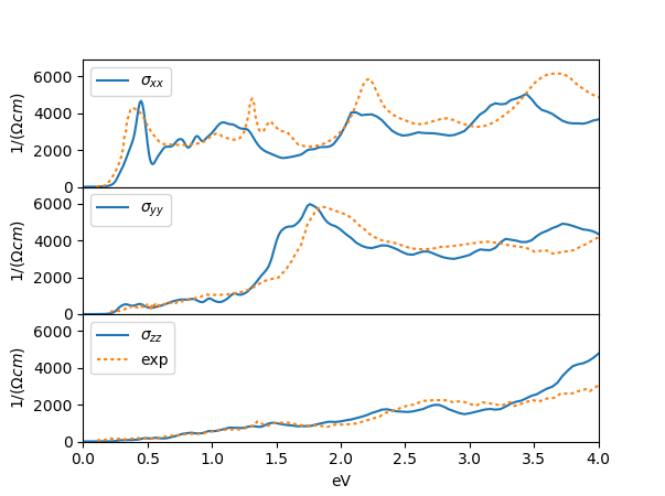 Note that the high-frequency peaks are somewhat red-shifted, which is
quite common feature of dft-type calculations, as the high-frequency
orbitals are somewhat less precisely predicted by dft, and are not
corrected by dmft.
Note that the high-frequency peaks are somewhat red-shifted, which is
quite common feature of dft-type calculations, as the high-frequency
orbitals are somewhat less precisely predicted by dft, and are not
corrected by dmft.