
Tutorial 5: Ce-alpha to gamma transition.
The alpha to gamma transition in Cerium is isostructural, i.e., the
volume of the fcc structure changes for 14%, and there is enormous
difference in coherence scale between the two phases.
On average, Cerium has one electron in the 4f-shell, which we will
treat dynamically with DMFT. To contrast the difference between the
two phases, we will explain the process for calculating both phases in
parallel. The only difference for the two phases is the different lattice
constant, entered in the structure file.
The first step is to make a DFT calculation to get a good
charge density. Copy
the Ce_alpha.struct file into
directory with name Ce_alpha, and run
Choose default
options in Wien2k setup. We can choose a small number of k-points
(200) at first to converge LDA/GGA run. Next, add spin-orbit
coupling by running
and then rerun LDA/GGA by
Next increase the number of k-points to a large number (say
5000). For alpha phase, which has a narrow Kondo peak, it is advisable
to use even more k-points, like 10000. Then rerun LDA/GGA once more
Exactly the
same procedure should be repeated for gamma phase, with the structure
file Ce_gamma.struct.
Note that if you want to compare the total free energies between the two
phases, you have to make sure that the muffin-tin sphere for both
calculations is the same (check RMT in case.struct).
Once the DFT calculation is done, we have a good charge
density to start a DMFT calculation. The next step is to initialize
the DMFT calculation using
There are 1 atoms in the unit cell:
  1 Ce
Specify correlated atoms (ex: 1-4,7,8): 1
We choose the Ce atom to be treated as a correlated.
For each atom, specify correlated orbital(s) (ex: d,f):
  1 Ce: f
Specify qsplit for each correlated orbital (default = 0):
    Qsplit  Description
------  ------------------------------------------------------------
     0  average GF, non-correlated
     1  |j,mj> basis, no symmetry, except time reversal (-jz=jz)
    -1  |j,mj> basis, no symmetry, not even time reversal (-jz=jz)
     2  real harmonics basis, no symmetry, except spin (up=dn)
    -2  real harmonics basis, no symmetry, not even spin (up=dn)
     3  t2g orbitals
    -3  eg orbitals
     4  |j,mj>, only l-1/2 and l+1/2
     5  axial symmetry in real harmonics
     6  hexagonal symmetry in real harmonics
     7  cubic symmetry in real harmonics
     8  axial symmetry in real harmonics, up different than down
     9  hexagonal symmetry in real harmonics, up different than down
    10  cubic symmetry in real harmonics, up different then down
    11  |j,mj> basis, non-zero off diagonal elements
    12  real harmonics, non-zero off diagonal elements
    13  J_eff=1/2 basis for 5d ions, non-magnetic with symmetry
    14  J_eff=1/2 basis for 5d ions, no symmetry
------  ------------------------------------------------------------
  1  Ce-1 f: 4
Specify projector type (default = 2):
  Projector  Description
------  ------------------------------------------------------------
     1  projection to the solution of Dirac equation (to the head)
     2  projection to the Dirac solution, its energy derivative,
          LO orbital, as described by P2 in PRB 81, 195107 (2010)
     4  similar to projector-2, but takes fixed number of bands in
          some energy range, even when chemical potential and
          MT-zero moves (folows band with certain index)
     5  fixed projector, which is written to projectorw.dat. You can
        generate projectorw.dat with the tool wavef.py
------  ------------------------------------------------------------
> 5
Do you want to group any of these orbitals into cluster-DMFT problems? (y/n): n
Enter the correlated problems forming each unique correlated
problem, separated by spaces (ex: 1,3 2,4 5-8): 1
Range (in eV) of hybridization taken into account in impurity
problems; default -10.0, 10.0: <ENTER>
Perform calculation on real; or imaginary axis? (r/i): i
Is this a spin-orbit run? (y/n): y
Next create a new folder, and when in that folder, use the
command
dmft_copy.py <lda_results_directory>
Next, copy the params.dat file,
which has the content
solver         =  'CTQMC'   # impurity solver
DCs            =  'nominal' # double counting scheme

max_dmft_iterations = 1     # number of iteration of the dmft-loop only
max_lda_iterations  = 100   # number of iteration of the LDA-loop only
finish         =  50        # number of iterations of full charge loop (1 = no charge self-consistency)

ntail          =  300       # on imaginary axis, number of points in the tail of the logarithmic mesh

cc             =  2e-6      # the charge density precision to stop the LDA+DMFT run
ec             =  2e-6      # the energy precision to stop the LDA+DMFT run

recomputeEF    = 1          # Recompute EF in dmft2 step. If recomputeEF = 2, it tries to find an insulating gap.
# mix_delta    = 0.5        # uncomment, if experience instability

# Impurity problem number 0
iparams0={"exe"                : ["ctqmc"              , "# Name of the executable"],
          "U"                  : [6.0                  , "# Coulomb repulsion (F0)"],
          "J"                  : [0.7                  , "# Coulomb repulsion (F0)"],
          "nc"                 : [[0,1,2,3]            , "# Impurity occupancies"],
          "beta"               : [100                  , "# Inverse temperature"],
          "svd_lmax"           : [25                   , "# We will use SVD basis to expand G, with this cutoff"],
          "M"                  : [10e6                 , "# Total number of Monte Carlo steps"],
          "mode"               : ["SH"                 , "# We will use self-energy sampling, and Hubbard I tail"],
          "nom"                : [200                  , "# Number of Matsubara frequency points sampled"],
          "tsample"            : [300                  , "# How often to record measurements"],
          "GlobalFlip"         : [1000000              , "# How often to try a global flip"],
          "warmup"             : [3e5                  , "# Warmup number of QMC steps"],
          "atom_Nmax"          : [100                  , "# Maximun size of the block in generatic atomic states"],
          "nf0"                : [1.0                  , "# Nominal occupancy nd for double-counting"],
}
The other important difference compared to previous calculations on
d systems is in two additional
parameters, which both control the exact diagonalization of the
atom. These parameters are specific to f-systems, and have no effect
in d systems:
nc=[0,1,2,3]
specifies that we will take into account
only a finite number of valences, namely Ce f0, f1,
f2, and f3 configurations. This considerably
speeds up the calculation, and it does not reduce the precision, as
the probability for f4 is below numeric precision.
atom_Nmax=100
specifies that if a block of atomic
eigenstates has dimension more than 100, it should be cut to size
100. This does not have any effect in Ce, as the largest block in
f3 configuration is 41-dimensional. But this improves the
speed considerably in heavier lanthanides and actinides, where these
blocks are much larger.
To proceed, one should create a blank self-energy on imaginary axis by a command
Alternatively, if an approximate self-energy exists, one can just copy
sig.inp approximate self-energy to the current directory. To restart
from previous run, one needs to copy also EF.dat file (chemical
potential) and "case.clmsum" (charge density).
Moreover, to allow the impurity to restart from the previous calculation,
one can also copy imp.0/status.xxx files, which contain the
last configuration of the impurity solver. We also provide
status_1.tgz, status_2.tgz, and status_3.tgz
files, which contain status files from previous steps, from one, two
and three steps before. This is useful when we want to restart from a
status from a few steps ago, in case the calculation goes in the wrong
direction.
Now we have all files prepared, and we can submit the job. The
submit-script should invoke python
script "$WIEN_DMFT_ROOT/run_dmft.py". Do not forget to
prepare mpi_prefix.dat file before invoking the python
script.
Once the DFT+DMFT is running, monitor its status by checking the
log files
- at the to level: info.iterate, :log,
case.scf, case.dayfile, dmft_info.out.
- dmft1 step can be monitored by checking dmft1_info.out and
Ce_alpha.outputdmf1
- impurity can be monitored by checking imp.0/ctqmc.log.xxx, imp.0/nohup_imp.out.000
imp.0/Sig.out.xxx and imp.0/Gf.out.xxx
- dmft2 step is best monitored through dmft2_info.out and
Ce_alpha.outputdmf2
To check what is the distribution of perturbation orders, we can plot
imp.0/histogram.dat, which should be
gaussian, and should look like:
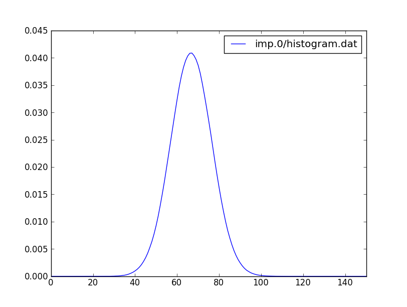 This
show the distribution of the perturbation order, which is related to
the kinetic energy. (In the older versions of the code, one had to
specify the maximum perturbation order allowed (Nmax), but in the new
version of the code, this is not needed).
This
show the distribution of the perturbation order, which is related to
the kinetic energy. (In the older versions of the code, one had to
specify the maximum perturbation order allowed (Nmax), but in the new
version of the code, this is not needed).
We can also check what is the probability for each atomic state, i.e.,
probability that a Ce-f electron is in any of the atomic states. This
information is written in imp.0/Probability.dat. The first and the
second column correspond to the index of each state, as defined in
actqmc.cix ( which enumerates all atomic states). The third column
is the probability for a state. Note that the first column is the
index of the block of atomic state as specified in actqmc.cix index
table. As each block of atomic states is in general multidimensional
(the corresponding energies are listed in a single row of the
actqmc.cix file), we need the second index.
Here is the plot of probability for
first 106 states:
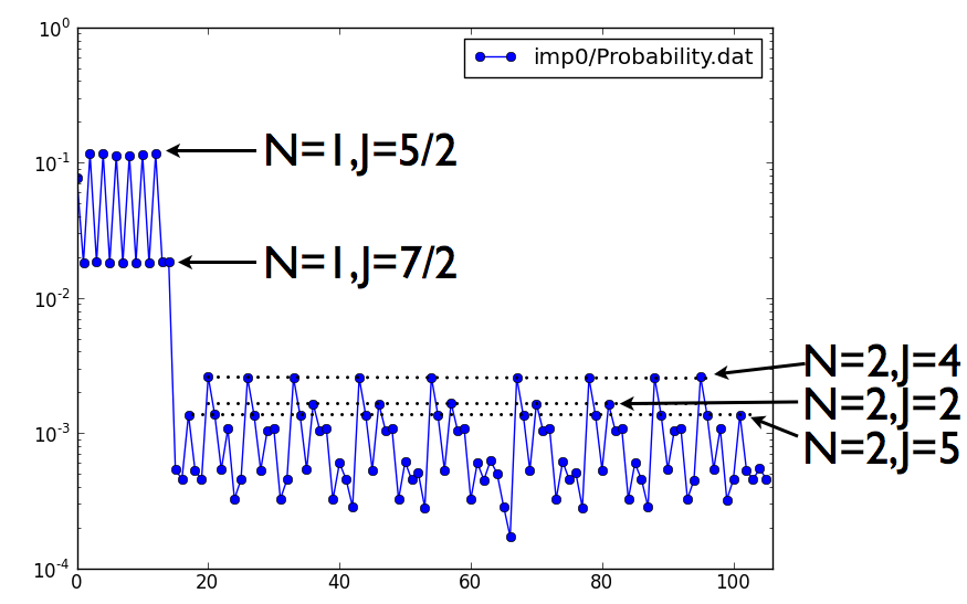 The
first state corresponds to the empty 4f ion. The next 14 states (from
1..14) correspond to nominal occupancy N=1, and the values between 15
and 106 correspond to occupancy N=2. At N=1, there are two sets of
probabilities, 6 take the value around 0.11, and 8 take the value of
0.018. The first and the second set corresponds to j=5/2 and j=7/2
multiplet, respectively. The next 92 states, which correspond to
occupancy N=2, have probablity around 1e-3. They can be grouped into
multiplets, the lowest being J=4, followed by J=2 and J=5. Notice that
the lowest multiplet satisfies Hunds rules (largest S=1, largest L=5,
and J=L-S=4). Notice also that although alpha-Ce is a very itinerant
metal, the projection to the atomic states still satisfies atomic
rules, such as Hunds rules.
The cumulative probability for N=2 states is around 0.086. Compare
this to N=1 probability of 0.836, and N=0 probability of 0.077. The
next 364 states correspond to N=3 occupancy, and their histogram looks
like:
The
first state corresponds to the empty 4f ion. The next 14 states (from
1..14) correspond to nominal occupancy N=1, and the values between 15
and 106 correspond to occupancy N=2. At N=1, there are two sets of
probabilities, 6 take the value around 0.11, and 8 take the value of
0.018. The first and the second set corresponds to j=5/2 and j=7/2
multiplet, respectively. The next 92 states, which correspond to
occupancy N=2, have probablity around 1e-3. They can be grouped into
multiplets, the lowest being J=4, followed by J=2 and J=5. Notice that
the lowest multiplet satisfies Hunds rules (largest S=1, largest L=5,
and J=L-S=4). Notice also that although alpha-Ce is a very itinerant
metal, the projection to the atomic states still satisfies atomic
rules, such as Hunds rules.
The cumulative probability for N=2 states is around 0.086. Compare
this to N=1 probability of 0.836, and N=0 probability of 0.077. The
next 364 states correspond to N=3 occupancy, and their histogram looks
like:
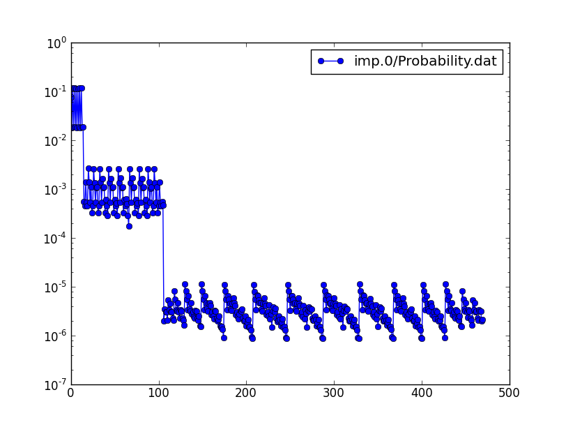 Typical probability of N=3 state is 1e-6, and cumulative probability
is 0.0012. Clearly, the probability falls off very rapidly with particle
number N, hence we can safely restrict occupancy in params.dat file to
nc=[0,1,2,3].
Typical probability of N=3 state is 1e-6, and cumulative probability
is 0.0012. Clearly, the probability falls off very rapidly with particle
number N, hence we can safely restrict occupancy in params.dat file to
nc=[0,1,2,3].
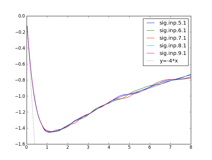
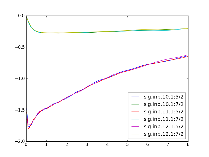
In the next plots, we show the self-energy on imaginary axis for both
alpha and gamma phase or Cerium.
We can monitor self-energy during the self-consistent run. After 3
DMFT iterations, the self-energy of alpha-Cerium is almost converged,
and we see that it does not change much between iteration 5-9. The
slope of imaginary part of the the 5/2 self-energy is dSigma/dw~4,
which gives mass enhancement of m*/m~5, i.e., the quasiparticle peak
is roughly 5-times narrower than in DFT.
The gamma-phase of Cerium is in local moment regime, where the
scattering rate at low energy is very large (bad metal). Here we see
the imaginary part of 5/2 self-energy to reach 1.5eV.
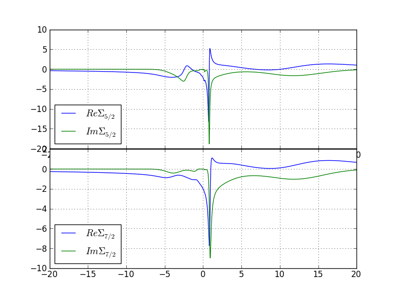
 Notice that the 7/2 self-enery is Fermi-liquid like, however, the 7/2
states have almost no weight at the Fermi level.
Notice that the 7/2 self-enery is Fermi-liquid like, however, the 7/2
states have almost no weight at the Fermi level.
To obtain the self-energy on the real axis, we need to do analytical
continuation from Matsubara to real axis. We will use maximum-entropy
method on auxiliary quantity
Gauxiliary=1/(omega-Sigma+Sigmainfty).
First we take the average of the sig.inp files from
the last few steps (in order to reduce the noise) by
saverage.py sig.inp.[5-9].1
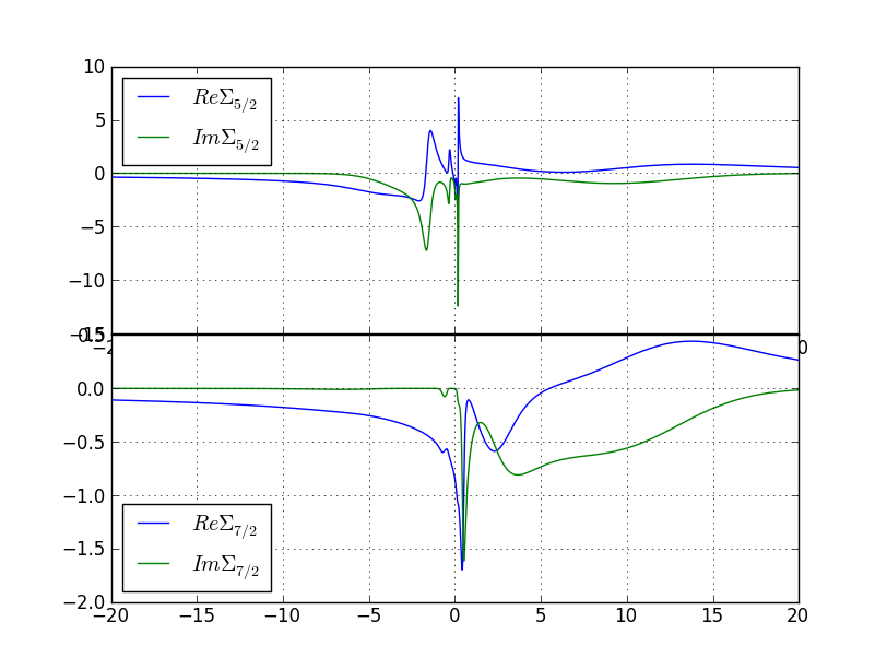
 and for the gamma phase to this plot:
Now we need to make one last dmft1 calculation in order to
obtain the Green's function and DOS on the real axis. Create a new
directory, and use
dmft_copy.py <dmft_results>
x lapw0 -f alpha-Ce
x_dmft.py lapw1
x_dmft.py lapwso
x_dmft.py dmft1
 and for gamma-phase similar to this plot:
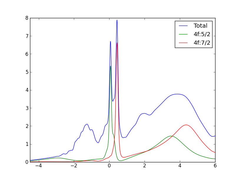
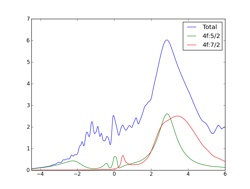 The partial 5/2 and 7/2 DOS can be obtained from case.gc1, while the
total DOS and projected 4f-DOS can be obtained from case.cdos.
Note a huge difference in the strength of the quasiparticle peak near
the Fermi level between the two phases. Also note that the gamma-phase
is not stable at 116K (the temperature of our calculation), it is
stable only above 200K at zero pressure. This calculation would than
correspond to a metastable state. At higher temperature, the small
peak at EF in gamma-phase would be even broadener. Also note the
characteristic splitting of the quasiparticle peak in cerium into
three peaks, one below EF at roughly -SO energy, the 5/2 peak at the
EF, and 7/2 peak at +SO energy. This splitting becomes even more
pronounced in gamma phase because the huge quasiparticle peak in alpha
phase prevents a clear identification of peak at -SO.
The partial 5/2 and 7/2 DOS can be obtained from case.gc1, while the
total DOS and projected 4f-DOS can be obtained from case.cdos.
Note a huge difference in the strength of the quasiparticle peak near
the Fermi level between the two phases. Also note that the gamma-phase
is not stable at 116K (the temperature of our calculation), it is
stable only above 200K at zero pressure. This calculation would than
correspond to a metastable state. At higher temperature, the small
peak at EF in gamma-phase would be even broadener. Also note the
characteristic splitting of the quasiparticle peak in cerium into
three peaks, one below EF at roughly -SO energy, the 5/2 peak at the
EF, and 7/2 peak at +SO energy. This splitting becomes even more
pronounced in gamma phase because the huge quasiparticle peak in alpha
phase prevents a clear identification of peak at -SO.
Finally, let us resolve the spectra in momentum space. For that we
first need to prepare k-list. We can take one from Wien2k templated
for fcc crystal structure. We then run DFT by
x lapw1 -f alpha-Ce -band
x lapwso -f alpha-Ce -band
We also need to edit alpha-Ce.indmfl file to set the range in
frequency and make sure that matsubara is set to 0. We will use 400
frequency points on real axis in the energy window -4eV to 5eV, hence
the header of alpha-Ce.indmfl will look like that
9 34 1 5                              # hybridization band index nemin and nemax, renormalize for interstitials, projection type
1 0.025 0.025 400 -4.000000 5.000000  # matsubara, broadening-corr, broadening-noncorr, nomega, omega_min, omega_max (in eV)
Next, we compute DMFT eigenvalues by executing
Finally, we plot the spectral function by
invoking
If the spectra looks too dim, we can
adjust the intensity by adding an argument, which is smaller than 0.2,
for example
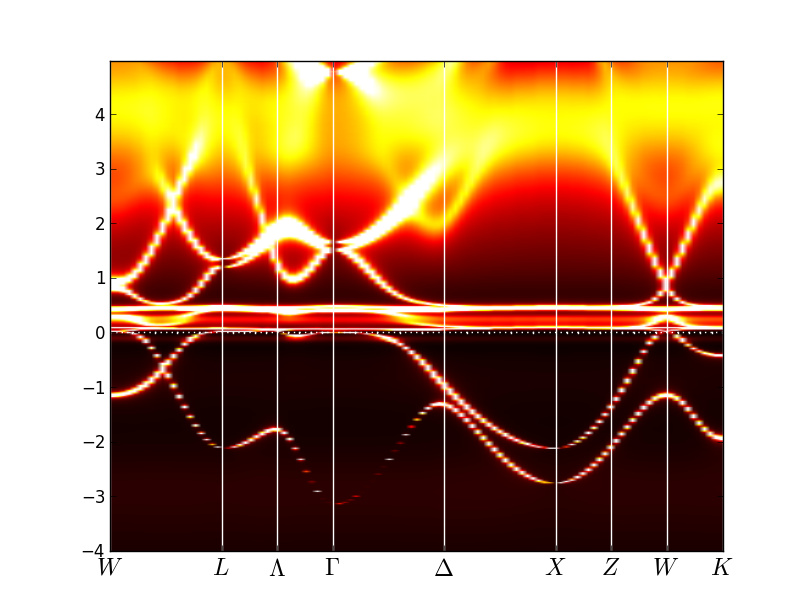
The spectra for the alpha phase should look like that:
 and for the gamma phase like that:
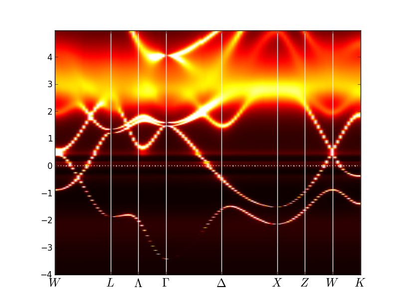 This clearly shows that in gamma phase the spectral features
associated with f-states loose intensity dramatically, while some
kinks in the spectra persist even in local moment regime. Also note
that the lower Hubbard band, which is located between -3eV and -2eV, is
very hard to identify in the spectra. The upper Hubbard band has much more
intensity and it is easier to see it, being centered at 3-4eV.
Note that the spectral weight distribution on the real axis is not
very precise, as it is obtained by maximum entropy method, which gives
only a rough approximation for the spectra on the real axis.
This clearly shows that in gamma phase the spectral features
associated with f-states loose intensity dramatically, while some
kinks in the spectra persist even in local moment regime. Also note
that the lower Hubbard band, which is located between -3eV and -2eV, is
very hard to identify in the spectra. The upper Hubbard band has much more
intensity and it is easier to see it, being centered at 3-4eV.
Note that the spectral weight distribution on the real axis is not
very precise, as it is obtained by maximum entropy method, which gives
only a rough approximation for the spectra on the real axis.