Tutorial 9: High-throughput functionality
This tutorial is on the two scripts that are provided for high
throughput type calculations within DFT+eDMFT. The scripts are
"cif2struct.py" and "cif2indmf.py". The first converts cif (or
magnetic mcif) file to proper structure file for wien2k calculation,
while the latter also prepares all necessary input files for eDMFT
calculation (as well as converts cif to structure file).
They require pymatgen
installation. The code has been tested with pymatgen version "2023.11.12" and
"2024.2.8".
The first script is cif2struct.py, which was already mentioned before.
It has several options, which are available through "-h" or "--help"
flag.
Options:
  -h, --help            show this help message and exit
  -w, --writek          weather to write case.klist_band high symmetry k-path
                        (default False)
  -N NKP, --Nkp=NKP     number of k-points along the high symmetry path
  -l LOG, --log=LOG     info file
  -n, --neigh           compute neighbors and evaluate Rmt
  -m, --magnet          should produce magnetic dft struct that allows broken
                        symmetry from mcif
  -H, --hexagonal       switches off hexagonal to rhombohedral conversion
  -p NDECIMALS, --ndecimals=NDECIMALS
                        precision when determining the equivalency of atoms we
                        take nn distance with precision ndecimals. Compatible
                        with w2k nn method.
  -R NRADIUS, --nradius=NRADIUS
                        How far in AA should nearest neighbors be checked.
                        Compatible with w2k nn method.
With "-N" we can increase or reduce the number of k-points. With -l we
can change the log filename, which is cif2struct.log by
default, and is very useful to read.
If the cif file is magnetic mcif file, we can switch on "-m" option to
produce input for magnetic calculation (no SO).
By default we convert hexagonal structures to rhombohedral as wien2k
would do it later in initialization. But we don't want to change
structure later, because in this case we also need to change local
axis again. The "-H" switch allows one to not perform this conversion.
We can also produce nearest neighbor list with "-n" and correctly set
RMT radius in structure file. But this neighbors list is crucial for
the second script, namely,
which produces a complete set of all
input files for dmft calculation, which are a good guess for a best set
of parameters.
The script takes many optional parameters:
Options:
  -h, --help            show this help message and exit
  -w, --writek          weather to write case.klist_band high symmetry k-path
                        (default False)
  -s, --so              is this with spin-orbit or not (default False)
  -r, --real            real axis sets matsubara to 0 in indmffile (default
                        False)
  -f, --fix             fix the chemical potential for Mott insulators
                        (default False)
  -N NKP, --Nkp=NKP     number of k-points along the high symmetry path
                        (default 300)
  -l LOG, --log=LOG     info file (default cif2struct.log)
  -c COR, --cor=COR     which atom types are correlated. all or 3,4 or 3-5 or
                        6-7 (default all)
  -d DC, --dc=DC        The type of double-counting: exact, exacty, exactd,
                        nominal (default exacty)
  -U COULOMBU, --U=COULOMBU
                        Coulomb U if we want to set it through input (default
                        None, set inside for each type)
  -J COULOMBJ, --J=COULOMBJ
                        Coulomb J if we want to set it through input (default
                        None, set inside for each type)
  -b BETA, --beta=BETA  inverse temperature (default 50/eV->232K)
  -M QMC_M, --QMC_M=QMC_M
                        Number of MC steps per core (default = 5M)
  -q QSPLIT, --qsplit=QSPLIT
                        qsplit (default = 2)
  -m, --magnet          should produce magnetic dft struct that allows broken
                        symmetry from mcif
  -H, --hexagonal       switches off hexagonal to rhombohedral conversion
  -p NDECIMALS, --ndecimals=NDECIMALS
                        precision when determining the equivalency of atoms we
                        take nn distance with precision ndecimals. Compatible
                        with w2k nn method.
  -R NRADIUS, --nradius=NRADIUS
                        How far in AA should nearest neighbors be checked.
                        Compatible with w2k nn method.
{3:["V","Cr","Mn","Fe","Co","Ni","Cu"],
 4:["Nb","Mo","Tc","Ru","Rh","Pd"],
 5:["Ta","W","Re","Os","Ir","Pt"],
 6:["Ce","Pr","Nd","Pm","Sm","Eu","Gd","Tb","Dy","Ho","Er","Tm","Yb","Lu"],
 7:["Th","Pa","U","Np","Pu","Am","Cm","Bk","Cf","Es","Fm","Md","No","Lr"]
}
Us={3: 10., 4: 8.0, 5: 7.0, 6: 6.0, 7: 6.0}
Js={3: 0.8, 4: 0.8, 5: 0.8, 6: 0.7, 7: 0.7}
     0  average GF, non-correlated
     1  |j,mj> basis, no symmetry, except time reversal (-jz=jz)
    -1  |j,mj> basis, no symmetry, not even time reversal (-jz=jz)
     2  real harmonics basis, no symmetry, except spin (up=dn)
    -2  real harmonics basis, no symmetry, not even spin (up=dn)
     3  t2g orbitals
    -3  eg orbitals
     4  |j,mj>, only l-1/2 and l+1/2
     5  axial symmetry in real harmonics
     6  hexagonal symmetry in real harmonics
     7  cubic symmetry in real harmonics
     8  axial symmetry in real harmonics, up different than down
     9  hexagonal symmetry in real harmonics, up different than down
    10  cubic symmetry in real harmonics, up different then down
    11  |j,mj> basis, non-zero off diagonal elements
    12  real harmonics, non-zero off diagonal elements
    13  J_eff=1/2 basis for 5d ions, non-magnetic with symmetry
    14  J_eff=1/2 basis for 5d ions, no symmetry
The harderst algorithm in this script is choosing the best local
coordinate axis on all correlated atoms, so that the hybridization
function has minimal off-diagonal components.
For that purpose, the script includes
localaxes.py script, which tries to guess the best polyhedra
surrounding the correlated atom, and from the polyhedra it tries to
determine the best local axis. It implements cube(8), octahedra(6),
tetrahedra(4), square-piramid(5), cuboctahedron (12), truncated
tetrahedron (12), peak-of-tetrahedron(3), peak-of-square-piramid(4),
peak-of-hexagonal-piramid(6), trigonal prism(6), planar quadrilateral
(4). In the bracket with quote the number of neighbors needed for each
polyhedra.
The script cif2indmf.py will produce case.struct, case.indmf, case.indmfl,
case.indmfi, params.dat, and with "-w" flag also
case.klist_band. Information is written to
cif2struct.log.
Three things are still needed for dmft run, namely,
- projectorw.dat file for projector=5,
- the band range in the top of case.indmfl, which is for now set to zero.
- nf0 in params.dat is set to number obtained from atomic configuration and
oxidation state guessed from the chemical formula. This is often not
precise enough
All these values can be obtained from converged dft run, hence the
third script
should be run after dft run is complete. It will write real space
projector to projectorw.dat. Next, it will check the band range
written in case.indmf in eV around the Fermi level, and convert
this number to integer band range obtained from case.energy files.
Finally, it will check the dft density matrix and guess the best density
nf0 for dmft double-counting, so that the starting point in
double-counting is excellent. Even when we use exact double
counting, we start with first guess that is proportional to this
nf0 value, because we don't have impurity occupancy yet.
Finally, after init_proj.py has been run, we need to call
to produce a good guess for self-energy (best s_oo and Edc).
The complete list of commands for high-throughput calculation could thus be
  $WIEN_DMFT_ROOT/cif2indmf.py -w case.cif >& nohup_init.dat
  echo "mpirun -n $NSLOTS" > mpi_prefix.dat
  echo "mpirun -n $NSLOTS" > mpi_prefix.dat2
  $WIENROOT/init_lapw -b -red 0 -vxc 5 -ecut -7.0  -numk 2000 >> nohup_init.dat
  $WIEN_DMFT_ROOT/run_dft.py >> nohup_dft.dat
  $WIEN_DMFT_ROOT/init_proj.py  -a >> nohup_init.dat
  $WIEN_DMFT_ROOT/szero.py >> nohup_init.dat
  $WIEN_DMFT_ROOT/run_dmft.py >& nohup_dmft.dat
Of course one could use less k-points to converg dft, and later
increase the number of k-points for dmft. But these details can be
easily added.
One should also check how off diagonal is the hybridization, by running
one dmft1 step with qsplit=12. Namely, qsplit=12 will produce all
off-diagonal hybridizations, which should be checked to be small. If
not, one could possibly run
$WIEN_DMFT_ROOT/findRot.py
to diagonalize hybridization on dft level before executing dmft. More
about this below in the case of RuO2.
Finally, we need to use a uniform choice of parameters for all
calculations. In the following we will select
U=10eV
J=0.8eV
DCs='exact'
qsplit=2
CoulombF='Ising'
This works quite well for 3d correlated compounds which are strongly
correlated. CoulombF='Full' is better, but is expensive.
For metals, like Fe superconductors, U should be somewhat
reduced. exact is a combination of exacty and
exactd double-counting. The first is a combination of yukawa and dielectric
screening that gives prescribed U and J, while the latter is purely
dielectric screening. While exacty is expected to be best in
many materials, it seems to be too short ranged in late TMO's, which
require more dielectric type screening. As a result exact is a
compromise that interpolated between exacty in early TMOs and
exactd in later TMOs.
We also added a new convergence criteria in the code. In the past the
outside DFT+DMFT loop would typically take finish number
of steps. By default, finish was set to 50. In the new
version of the code, we compute (nimp-nlatt)
at the point of the converged charge (DFT+DMFT charge is
converged) and than compare two successive impurity steps (always
taking converged real space charge). If the difference between two
successive steps is below treshold, we stop eDMFT. The variable to
set the treshold for convergence is called 'nc'.
We currently have three convergence criteria which need to be satisfied for
stoping the DFT+DMFT run:
- cc=1e-5 # the charge density precision to stop the eDMFT run
- ec=1e-5 # the total energy precision to stop the eDMFT run
- nc=5e-4 # the impurity difference to stop eDMFT run
If one preferes the behaviour in Python2 code, one would set nc to
very small number in params.dat
With this in mind, we rerun a few compounds discussed in previous
tutorials, and we will next present the results, so that user can
check if the code works correctly.
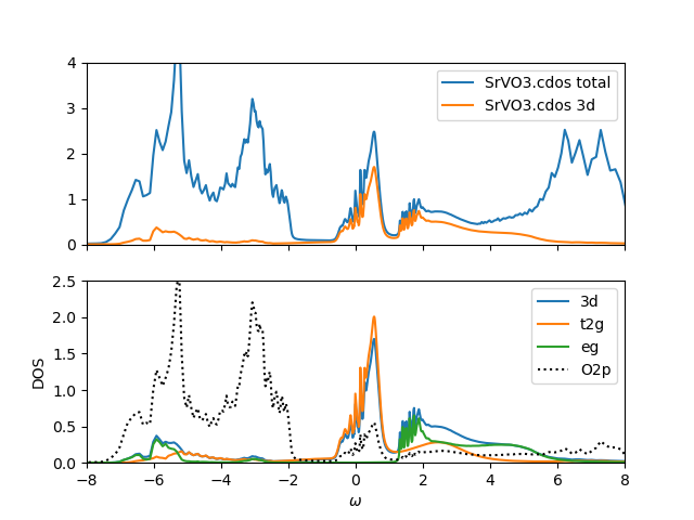
SrVO3
We rerun SrVO3 with these default parameter. Notice that
before we correlated only t2g orbitals and used smaller
U=8eV. Now we correlate both the t2g and eg orbitals and
with increased U=10eV, we produce similar spectra and similar
occupancies. For example, the t2g only occupancy was before
n_{t2g}=1.45, while the new calculation gives n_{t2g}=1.522 and
n_{eg}=0.715. The total 3d occupancy is much bigger n_{3d}=2.24, but
this is because we now count both the eg and t2g electrons.
The converged results in info.file is
    mu          Vdc            Etot     Ftot+T*Simp     Ftot+T*Simp       n_latt        n_imp      Eimp[0]     Eimp[-1]
8.661942    15.551639    -8710.159608    -8710.165781    -8710.158820     2.240679     2.237563    -0.085963    -1.448770
 These are similar than before, but correlations are now somewhat weaker. The mass
enhancement is now only around m*/m~2 as compared to m*/m~2.5 in t2g
only calculation. This is close, but if we wanted to get a better
agreement with previous t2g only calculation, we would need to further
reduce U in previous calculation. We notice however that
the calculations are much harder to converge now, because the typical
perturbation order is now around order 450 (extending beyond 500),
while in t2g only calculation, the typical order was 170 (extending to 230).
Finally, we show the hybridization function for t2g orbital:
 This is almost identical to previous t2g only calculation.
LaVO3
In one of the previous tutorials we have performed t2g-only
calculation for LaVO3, which it turned out to be Mott insulating
material with t2g occupancy close to 2, and Mott gap close to, but smaller
than 2eV. In this tutorial we correlated all 3d orbitals, and
automatically select the best local axis. You can check that
case.indmfl files has local rotation equivalent to the one we
produced in previous tutorial.
The self-consistent calculation with all 5d orbitals and larger U=10eV
produces similar results. However, there are also difference.
First we point out that the Mott gap can be numerically stabilized
with fixing the chemical potential. We thus change the flag in
params.dat file to
and than check in dmft_info.out or case.outputdmf2 file
that
is close to zero. If there is a gap, this number will be an integer,
and we must ensure it is not +1 or -1, but close to zero.
The converged values in info.iterate are:
       mu          Vdc            Etot     Ftot+T*Simp     Ftot+T*Simp       n_latt        n_imp      Eimp[0]     Eimp[-1]
10.803055    18.468704   -77383.390671   -77383.399318   -77383.389914     2.540813     2.543642     0.025545    -1.150281
      z^2                 x^2-y^2           xz                 yz                xy
mom=[0.2345946764349459,0.2332270335931207,0.7098984906471872,0.6736290320800302,0.6922923990033716,]
hence t2g occupancy is n_{t2g}=2.08, which is extremely close to
previous t2g only calculation with occupancy of n_{t2g}=2.1.
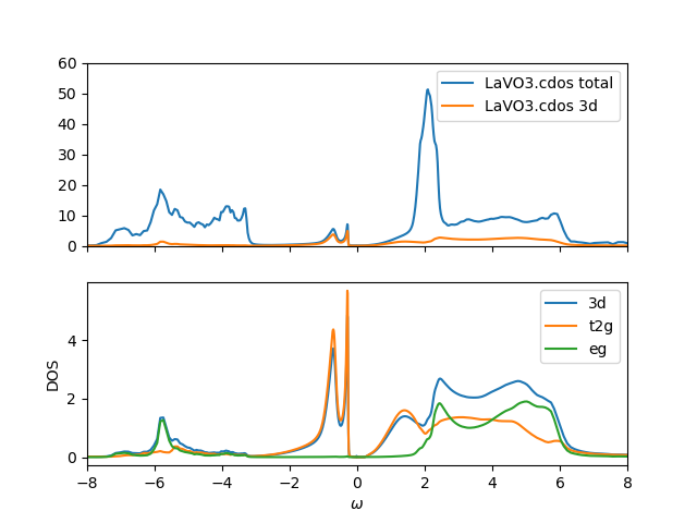
The local density of states is plotted below:
 It shows a small gap, and the lower Hubbard band split into Slatter
peak (first peak in the valence band) and more broad reminder of the
Hubbard band. This signals that the Mott gap is somewhat closer to the
Mott transition (but above), hence Slater peak is very pronounced. The
fact that we are close to the Mott transition was observed also
numerically, as convergence is much more challenging in this settings.
We notice that the eg-states have shifted slightly upward, similar as
in SrVO3. This is not surprising, as correlations should remove such
orbitals that are in empty orbital regime from the Fermi level.
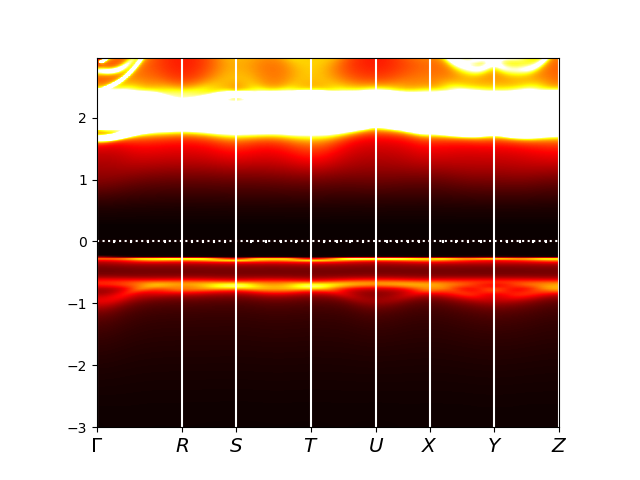
Finally, to check the size of the Mott gap we display the spectral
function. We notice that the size of the gap is very comparable to
what we have seen before (close to 2eV, but somewhat smaller than
2eV). We clearly see the splitting in the lower Hubbard band into
Slater peak and the rest. More importantly, the conduction band is
very different now. Before the conduction band started with eg states,
while now it starts with La-f states.
 Since La-f states are not treated as correlated, they might be misplaced, and it
is an interesting question if more precise calculation with
correlations on La-f states would increase the gap size or not.
FeSe
Finally, we also recompute the properties of FeSe with similar input
parameters. If we choose U=8eV and J=0.8eV with DCs=exact, we get
relaxed structure with z parameter around 0.3, and occupancy very
close to 6 (nd=6.07). This parameters predict very strong correlations, a bit
more than experiment shows.
When U=5eV and J=0.8eV with DCs=exact, we get a relaxes structure with z=0.281 and
occupancy nd=6.26, which is in
a reasonable agreement with experiment. We want to point out that
occupancy could be reduced by choosing DCs=exacty, which would
increase correlation strength and increase z. On the other hand,
choosing DCs=exactd would do the opposite, decrease the occupancy and
decrease correlations and structural parameter z. Increase of Hund's
coupling has similar effect in decreasing occupancy and increasing
correlation strengt. Here is the table that demonstrates the
sensitivity of the results with these parameters.
| U=5eV |
J=0.7eV |
J=0.8eV |
| DCs='exact' |
z=0.270, nd=6.32 |
z=0.281, nd=6.26 |
|
| DCs='exacty' |
z=0.300, nd=6.02 |
z=0.306, nd=5.95 |
Notice that J and DCs are even more crucial parameters than U in this case.
This is because FeSe is at the verge of selective Mott differentiation,
and therefore this strong sensitivity with small variation of
parameters.
RuO2 as Altermagnet
In this section we will demonstrate how to run eDMFT code for magnetic
materials, in this case altermagnet RuO2. This run will be done
without SO coupling, because this is the best way to distinguish
between altermagnets and other antiferromagnets that have SO induced
splitting of bands.
We start by downloading magnetic cif file from Bilbao
Crystallographic Server (RuO2 mcif
appears under number 0.607). For the purpose of this exercise we will
call it 0_607_RuO2.mcif.
First we will generate all eDMFT input files with cif2indmf.py
script. This script takes many options, which are listed with "-h" or
"--help" option:
Options:
  -h, --help            show this help message and exit
  -w, --writek          weather to write case.klist_band high symmetry k-path
                        (default False)
  -s, --so              is this with spin-orbit or not (default False)
  -r, --real            real axis sets matsubara to 0 in indmffile (default
                        False)
  -f, --fix             fix the chemical potential for Mott insulators
                        (default False)
  -N NKP, --Nkp=NKP     number of k-points along the high symmetry path
                        (default 300)
  -l LOG, --log=LOG     info file (default cif2struct.log)
  -c COR, --cor=COR     which atom types are correlated. all or 3,4 or 3-5 or
                        6-7 (default all)
  -d DC, --dc=DC        The type of double-counting: exact, exacty, exactd,
                        nominal (default exacty)
  -U COULOMBU, --U=COULOMBU
                        Coulomb U if we want to set it through input (default
                        None, set inside for each type)
  -J COULOMBJ, --J=COULOMBJ
                        Coulomb J if we want to set it through input (default
                        None, set inside for each type)
  -b BETA, --beta=BETA  inverse temperature (default 50/eV->232K)
  -M QMC_M, --QMC_M=QMC_M
                        Number of MC steps per core (default = 5M)
  -q QSPLIT, --qsplit=QSPLIT
                        qsplit (default = 2)
  -m, --magnet          should produce magnetic dft struct that allows broken
                        symmetry from mcif
  -H, --hexagonal       switches off hexagonal to rhombohedral conversion
  -p NDECIMALS, --ndecimals=NDECIMALS
                        precision when determining the equivalency of atoms we
                        take nn distance with precision ndecimals. Compatible
                        with w2k nn method.
  -R NRADIUS, --nradius=NRADIUS
                        How far in AA should nearest neighbors be checked.
                        Compatible with w2k nn method.
We will execute:
cif2indmf.py -w -m -U 6.0 0_607_RuO2.mcif
0_607_RuO2.struct
0_607_RuO2.indmfi
0_607_RuO2.indmfl
0_607_RuO2.indmfldn
0_607_RuO2.klist_band
params.dat
cif2struct.log
It is very useful to read cif2struct.log, which explains the algorithm
of generating all these files.
First it prints the structure read from cif file:
structure directly from given input cif file
---------------------------------------------
ca= 4.492 cb= 4.492 cc= 3.1061 calpha= 90.0 cbeta= 90.0 cgamma= 90.0
sgname= P  4_2/m  n  m sgnum= 136 ssetting= None
  1 Ru       0.000000, 0.000000, 0.000000
  2 O        0.305580, 0.305580, 0.000000
Full Formula (Ru2 O4)
Reduced Formula: RuO2
abc   :   4.492000   4.492000   3.106100
angles:  90.000000  90.000000  90.000000
pbc   :       True       True       True
Sites (6)
  #  SP          a        b    c    magmom
---  ----  -------  -------  ---  --------
  0  Ru    0        0        0        0.05
  1  Ru    0.5      0.5      0.5     -0.05
  2  O     0.30558  0.30558  0        0
  3  O     0.80558  0.19442  0.5      0
  4  O     0.19442  0.80558  0.5      0
  5  O     0.69442  0.69442  0        0
Number of symmetry operations available= 16
magnetic cif= True
0 : Time=1 I
 1 0 0 0.00000000
 0 1 0 0.00000000
 0 0 1 0.00000000
1 : Time=1 R
 1 0 0 0.50000000
 0-1 0 0.50000000
 0 0-1 0.50000000
2 : Time=1 R
-1 0 0 0.50000000
 0 1 0 0.50000000
 0 0-1 0.50000000
3 : Time=1 R
-1 0 0 0.00000000
 0-1 0 0.00000000
 0 0 1 0.00000000
4 : Time=1 P
-1 0 0 0.00000000
 0-1 0 0.00000000
 0 0-1 0.00000000
5 : Time=1 R
-1 0 0 0.50000000
 0 1 0 0.50000000
 0 0 1 0.50000000
6 : Time=1 R
 1 0 0 0.50000000
 0-1 0 0.50000000
 0 0 1 0.50000000
7 : Time=1 R
 1 0 0 0.00000000
 0 1 0 0.00000000
 0 0-1 0.00000000
8 : Time=-1 R
 0-1 0 0.50000000
 1 0 0 0.50000000
 0 0 1 0.50000000
9 : Time=-1 R
 0 1 0 0.50000000
-1 0 0 0.50000000
 0 0 1 0.50000000
10 : Time=-1 R
 0 1 0 0.00000000
 1 0 0 0.00000000
 0 0-1 0.00000000
11 : Time=-1 R
 0-1 0 0.00000000
-1 0 0 0.00000000
 0 0-1 0.00000000
12 : Time=-1 R
 0 1 0 0.50000000
-1 0 0 0.50000000
 0 0-1 0.50000000
13 : Time=-1 R
 0-1 0 0.50000000
 1 0 0 0.50000000
 0 0-1 0.50000000
14 : Time=-1 R
 0-1 0 0.00000000
-1 0 0 0.00000000
 0 0 1 0.00000000
15 : Time=-1 R
 0 1 0 0.00000000
 1 0 0 0.00000000
 0 0 1 0.00000000
Next few lines show how symmetry operations split the magnetic
symmetry operations to those that are present for spin-up (or
spin-down) only calculation. If operation flips spins, it should be
removed in spin-up calculation only. If it preserves the spin, it is
kept.
Ru[0] [0. 0. 0.] M[0]= [0.   0.   0.05]
Ru[1] [0.5 0.5 0.5] M[1]= [ 0.    0.   -0.05]
Group[1] applied to r[1]= [0.5 0.5 0.5] and M[1]= [0.0, 0.0, -0.05]  gives r[0]= [0. 0. 0.]  and M[0]= [0.0, 0.0, 0.05]
Molap= -1.0
Since moments are different ig= 1 should be removed flipped= {1: 0}
Group[2] applied to r[1]= [0.5 0.5 0.5] and M[1]= [0.0, 0.0, -0.05]  gives r[0]= [0. 0. 0.]  and M[0]= [0.0, 0.0, 0.05]
Molap= -1.0
Since moments are different ig= 2 should be removed flipped= {1: 0}
Group[5] applied to r[1]= [0.5 0.5 0.5] and M[1]= [0.0, 0.0, -0.05]  gives r[0]= [0. 0. 0.]  and M[0]= [0.0, 0.0, 0.05]
Molap= -1.0
Since moments are different ig= 5 should be removed flipped= {1: 0}
Group[6] applied to r[1]= [0.5 0.5 0.5] and M[1]= [0.0, 0.0, -0.05]  gives r[0]= [0. 0. 0.]  and M[0]= [0.0, 0.0, 0.05]
Molap= -1.0
Since moments are different ig= 6 should be removed flipped= {1: 0}
Group[8] applied to r[1]= [0.5 0.5 0.5] and M[1]= [0.0, 0.0, -0.05]  gives r[0]= [0. 0. 0.]  and M[0]= [0.0, 0.0, 0.05]
Molap= -1.0
Since moments are different ig= 8 should be removed flipped= {1: 0}
Group[9] applied to r[1]= [0.5 0.5 0.5] and M[1]= [0.0, 0.0, -0.05]  gives r[0]= [0. 0. 0.]  and M[0]= [0.0, 0.0, 0.05]
Molap= -1.0
Since moments are different ig= 9 should be removed flipped= {1: 0}
Group[12] applied to r[1]= [0.5 0.5 0.5] and M[1]= [0.0, 0.0, -0.05]  gives r[0]= [0. 0. 0.]  and M[0]= [0.0, 0.0, 0.05]
Molap= -1.0
Since moments are different ig= 12 should be removed flipped= {1: 0}
Group[13] applied to r[1]= [0.5 0.5 0.5] and M[1]= [0.0, 0.0, -0.05]  gives r[0]= [0. 0. 0.]  and M[0]= [0.0, 0.0, 0.05]
Molap= -1.0
Since moments are different ig= 13 should be removed flipped= {1: 0}
Starting anew with ii=1 grp= [[0], [1]]
groups for magnetic atoms= [[[0], [1]]]
indx_by_element {'Ru': [0, 1], 'O': [2, 3, 4, 5]}
starting with groups for magnetic atoms= [[[0], [1]], [[2, 3, 4, 5]]]
We apply all symmetry operations, and see that operation
[1,2,5,6,8,9,12,13] transform Ru[1] to Ru[0], and also flip the spin
(as they should),
while the rest of the operations [0,3,4,7,10,11,14,15] don't flip spins,
and they do not mix Ru[0] with Ru[1] with opposite spin, hence are
preserved in our calculation.
Next we produce a list of all magnetic atoms that form equivalent
group. We call that "groups for magnetic atoms", which is
"[[[0],[1]]]". It means that atom 0 and 1 are different. If the list
is "[[[0,1]]]" they would be considered equivalent.
The non-magnetic atoms are first considered to be equivalent if they
correspond to the same element. Since we only have oxygens at position
2,3,4,5, they are all considered equivalent for now, i.e.,
[2,3,4,5]. "indx_by_element" also shows which elements have which
successive number in the structure.
Next we print for each atom which symmetry operations transforms ups
into down spins. Here Ru[1] is transformed into Ru[0] and the
following symmetry operations flip the spin"
atoms which are flipped of each other:
1->0
    T=1
    R= 1, 0, 0
       0,-1, 0
       0, 0,-1
    T=1
    R=-1, 0, 0
       0, 1, 0
       0, 0,-1
    T=1
    R=-1, 0, 0
       0, 1, 0
       0, 0, 1
    T=1
    R= 1, 0, 0
       0,-1, 0
       0, 0, 1
    T=-1
    R= 0,-1, 0
       1, 0, 0
       0, 0, 1
    T=-1
    R= 0, 1, 0
      -1, 0, 0
       0, 0, 1
    T=-1
    R= 0, 1, 0
      -1, 0, 0
       0, 0,-1
    T=-1
    R= 0,-1, 0
       1, 0, 0
       0, 0,-1
symmetry operations that need to be removed= {1, 2, 5, 6, 8, 9, 12, 13}
Symmetry operations left:
0 : Time=1 I
 1 0 0 0.00000000
 0 1 0 0.00000000
 0 0 1 0.00000000
1 : Time=1 R
-1 0 0 0.00000000
 0-1 0 0.00000000
 0 0 1 0.00000000
2 : Time=1 P
-1 0 0 0.00000000
 0-1 0 0.00000000
 0 0-1 0.00000000
3 : Time=1 R
 1 0 0 0.00000000
 0 1 0 0.00000000
 0 0-1 0.00000000
4 : Time=-1 R
 0 1 0 0.00000000
 1 0 0 0.00000000
 0 0-1 0.00000000
5 : Time=-1 R
 0-1 0 0.00000000
-1 0 0 0.00000000
 0 0-1 0.00000000
6 : Time=-1 R
 0-1 0 0.00000000
-1 0 0 0.00000000
 0 0 1 0.00000000
7 : Time=-1 R
 0 1 0 0.00000000
 1 0 0 0.00000000
 0 0 1 0.00000000
Hence, we keep T[1]==C2(z), T[2]==inversion=P, T[4]==C2(110),
and their combinations: T[3]=C2(z)*P, T[6]=C2(1,1,0)*P,
T[5]=C2(1,1,0)*C2(z), T[7]=C2(1,1,0)*C2(z)*P.
We dropped C2(x)+(1/2,1/2,1/2), C2(y)+(1/2,1/2,1/2), C2(x)*P+(1/2,1/2,1/2), C2(y)*P+(1/2,1/2,1/2), C4++(1/2,1/2,1/2), C4-(z)+(1/2,1/2,1/2),
C4+(z)*P+(1/2,1/2,1/2), C4-(z)*P+(1/2,1/2,1/2), because they were
transforming spin-up Ru in spin-down Ru.
Next we determine equivalency for non-magnetic atoms using shells of
neighboring atoms as a test. This algorithm mirrors w2k-nn algorithm,
which also looks at all neighbors to determine equivalency.
At the first iteration we have the following atoms and their neighbors:
Going over all neighbors to determine equivalency:
....
neigbors of inequivalent atom types after iteration 1
   Ru1 ['1.941 O1 O1', '1.984 O1 O1 O1 O1', '3.106 Ru1 Ru1', '3.408 O1 O1 O1 O1', '3.536 Ru2 Ru2 Ru2 Ru2 Ru2 Ru2 Ru2 Ru2', '3.663 O1 O1 O1 O1', '4.034 O1 O1 O1 O1 O1 O1 >
   Ru2 ['1.941 O1 O1', '1.984 O1 O1 O1 O1', '3.106 Ru2 Ru2', '3.408 O1 O1 O1 O1', '3.536 Ru1 Ru1 Ru1 Ru1 Ru1 Ru1 Ru1 Ru1', '3.663 O1 O1 O1 O1', '4.034 O1 O1 O1 O1 O1 O1 >
   O1 ['1.941 Ru1', '1.984 Ru2 Ru2', '2.47 O1', '2.776 O1 O1 O1 O1 O1 O1 O1 O1', '3.106 O1 O1', '3.254 O1 O1', '3.408 Ru1 Ru1', '3.663 Ru1 Ru1', '3.882 O1', '3.969 O1 O1>
atom[ 3] with name=O1 neigbr= ['1.941 Ru2', '1.984 Ru1 Ru1', '2.47 O1', '2.776 O1 O1 O1 O1 O1 O1 O1 O1', '3.106 O1 O1', '3.254 O1 O1', '3.408 Ru2 Ru2', '3.663 Ru2 Ru2', >
atom[ 3] with name=O1 expect= ['1.941 Ru1', '1.984 Ru2 Ru2', '2.47 O1', '2.776 O1 O1 O1 O1 O1 O1 O1 O1', '3.106 O1 O1', '3.254 O1 O1', '3.408 Ru1 Ru1', '3.663 Ru1 Ru1', >
   Ru1 ['1.941 O1 O1', '1.984 O2 O2 O2 O2', '3.106 Ru1 Ru1', '3.408 O1 O1 O1 O1', '3.536 Ru2 Ru2 Ru2 Ru2 Ru2 Ru2 Ru2 Ru2', '3.663 O1 O1 O1 O1', '4.034 O2 O2 O2 O2 O2 O2 >
   Ru2 ['1.941 O2 O2', '1.984 O1 O1 O1 O1', '3.106 Ru2 Ru2', '3.408 O2 O2 O2 O2', '3.536 Ru1 Ru1 Ru1 Ru1 Ru1 Ru1 Ru1 Ru1', '3.663 O2 O2 O2 O2', '4.034 O1 O1 O1 O1 O1 O1 >
   O1 ['1.941 Ru1', '1.984 Ru2 Ru2', '2.47 O1', '2.776 O2 O2 O2 O2 O2 O2 O2 O2', '3.106 O1 O1', '3.254 O1 O1', '3.408 Ru1 Ru1', '3.663 Ru1 Ru1', '3.882 O1', '3.969 O1 O1>
   O2 ['1.941 Ru2', '1.984 Ru1 Ru1', '2.47 O2', '2.776 O1 O1 O1 O1 O1 O1 O1 O1', '3.106 O2 O2', '3.254 O2 O2', '3.408 Ru2 Ru2', '3.663 Ru2 Ru2', '3.882 O2', '3.969 O2 O2>
The other parameter that could potentially need to be changed is
"-R NRADIUS, --nradius=NRADIUS". By default we check neighbors up to
4.7A away from each atom. This is almost always enough to determine
equivalency. But if discrepancy between w2k-nn and this algorithm
occurs, one can check that this radius is sufficient. Note that in w2k we give
parameter in terms of number of shells for nn.
Finally, we determine the grouping of all atoms into equivalent
sets. We have:
mgroups= [[[0], [1]], [[2, 5], [3, 4]]]
In w2k we will list atoms consequently and O1 will appear as atoms
[2,3] and O2 as [4,5]. We now reorder atoms so as they will appear in
w2k structure file:
all_sites_order= [0, 1, 2, 5, 3, 4]
ATOM:   1 Ru  AT   0.00000   0.00000   0.00000=  0.00000   0.00000   0.00000
nn_distance= 1.9412419687117457 Rmt[0]= 1.037157052833468
  ATOM:  5 O     AT  -1.37267  -1.37267  -0.00000= -0.30558  -0.30558   0.00000 IS AWAY      1.941242      1.941242 ANG
  ATOM:  2 O     AT   1.37267   1.37267   0.00000=  0.30558   0.30558   0.00000 IS AWAY      1.941242      1.941242 ANG
  ATOM:  3 O     AT  -0.87333   0.87333  -1.55305= -0.19442   0.19442  -0.50000 IS AWAY      1.984286      1.984286 ANG
  ATOM:  3 O     AT  -0.87333   0.87333   1.55305= -0.19442   0.19442   0.50000 IS AWAY      1.984286      1.984286 ANG
  ATOM:  4 O     AT   0.87333  -0.87333  -1.55305=  0.19442  -0.19442  -0.50000 IS AWAY      1.984286      1.984286 ANG
  ATOM:  4 O     AT   0.87333  -0.87333   1.55305=  0.19442  -0.19442   0.50000 IS AWAY      1.984286      1.984286 ANG
  ATOM:  0 Ru    AT   0.00000   0.00000  -3.10610=  0.00000   0.00000  -1.00000 IS AWAY      3.106100      3.106100 ANG
  ATOM:  0 Ru    AT   0.00000   0.00000   3.10610=  0.00000   0.00000   1.00000 IS AWAY      3.106100      3.106100 ANG
  ATOM:  5 O     AT  -1.37267   3.11933   0.00000= -0.30558   0.69442   0.00000 IS AWAY      3.407999      3.407999 ANG
  ATOM:  2 O     AT  -3.11933   1.37267  -0.00000= -0.69442   0.30558   0.00000 IS AWAY      3.407999      3.407999 ANG
  ATOM:  5 O     AT   3.11933  -1.37267   0.00000=  0.69442  -0.30558   0.00000 IS AWAY      3.407999      3.407999 ANG
  ATOM:  2 O     AT   1.37267  -3.11933  -0.00000=  0.30558  -0.69442   0.00000 IS AWAY      3.407999      3.407999 ANG
  ATOM:  1 Ru    AT  -2.24600  -2.24600  -1.55305= -0.50000  -0.50000  -0.50000 IS AWAY      3.535675      3.535675 ANG
  ATOM:  1 Ru    AT  -2.24600  -2.24600   1.55305= -0.50000  -0.50000   0.50000 IS AWAY      3.535675      3.535675 ANG
  ATOM:  1 Ru    AT  -2.24600   2.24600  -1.55305= -0.50000   0.50000  -0.50000 IS AWAY      3.535675      3.535675 ANG
  ATOM:  1 Ru    AT  -2.24600   2.24600   1.55305= -0.50000   0.50000   0.50000 IS AWAY      3.535675      3.535675 ANG
  ATOM:  1 Ru    AT   2.24600  -2.24600  -1.55305=  0.50000  -0.50000  -0.50000 IS AWAY      3.535675      3.535675 ANG
  ATOM:  1 Ru    AT   2.24600  -2.24600   1.55305=  0.50000  -0.50000   0.50000 IS AWAY      3.535675      3.535675 ANG
  ATOM:  1 Ru    AT   2.24600   2.24600  -1.55305=  0.50000   0.50000  -0.50000 IS AWAY      3.535675      3.535675 ANG
  ATOM:  1 Ru    AT   2.24600   2.24600   1.55305=  0.50000   0.50000   0.50000 IS AWAY      3.535675      3.535675 ANG
  ATOM:  5 O     AT  -1.37267  -1.37267  -3.10610= -0.30558  -0.30558  -1.00000 IS AWAY      3.662824      3.662824 ANG
  ATOM:  5 O     AT  -1.37267  -1.37267   3.10610= -0.30558  -0.30558   1.00000 IS AWAY      3.662824      3.662824 ANG
  ATOM:  2 O     AT   1.37267   1.37267  -3.10610=  0.30558   0.30558  -1.00000 IS AWAY      3.662824      3.662824 ANG
  ATOM:  2 O     AT   1.37267   1.37267   3.10610=  0.30558   0.30558   1.00000 IS AWAY      3.662824      3.662824 ANG
The high-symmetry k-path proposed by pymatgen is give by
high symmetry kpath=
\Gamma  [0.0, 0.0, 0.0]
A       [0.5, 0.5, 0.5]
M       [0.5, 0.5, 0.0]
R       [0.0, 0.5, 0.5]
X       [0.0, 0.5, 0.0]
Z       [0.0, 0.0, 0.5]
Next we list information about the structure we just found, as
appropriate for findsym. In rare cases, in which the current algorithm
could fail, one could check with findsym, the appropriate space group
and new cif file. We list the information in the way that allows
direct copy/paste in findsym:
conventional unit cell (cif.w2k_coords) for finsym: https://stokes.byu.edu/iso/findsym.php:
cartesian coordinates of the basis vectors:
  4.49200   0.00000   0.00000
 -0.00000   4.49200   0.00000
  0.00000   0.00000   3.10610

Number of atoms in the unit cell:  6
Type of each atom in the unit cell: 1*Ru1  1*Ru2  2*O1  2*O2
  0.000000   0.000000   0.000000
  0.500000   0.500000   0.500000
  0.305580   0.305580   0.000000
  0.694420   0.694420   0.000000
  0.805580   0.194420   0.500000
  0.194420   0.805580   0.500000
After removing atoms not in primitive cell, we have the following cif.w2k_coords list:
name=Ru1 Z=44 [0. 0. 0.]
name=Ru2 Z=44 [0.5 0.5 0.5]
name=O1 Z=8 [0.30558 0.30558 0.     ]
name=O1 Z=8 [0.69442 0.69442 0.     ]
name=O2 Z=8 [0.80558 0.19442 0.5    ]
name=O2 Z=8 [0.19442 0.80558 0.5    ]
pymatgen_conventional=
  8.48865   0.00000   0.00000  ==a1
 -0.00000   8.48865   0.00000  ==a2
  0.00000   0.00000   5.86968  ==a3
paymatgen_Unit cell volume= 422.9524415348472

primitive or simple lattice

w2k_conventional=
  8.48865   0.00000   0.00000  ==a1
  0.00000   8.48865   0.00000  ==a2
  0.00000   0.00000   5.86968  ==a3
Unit cell volume= 422.95244153484725
Ortho= True
BR2=
  0.74019  -0.00000  -0.00000
  0.00000   0.74019  -0.00000
  0.00000   0.00000   1.07045

gbas=
  0.11780  -0.00000  -0.00000
  0.00000   0.11780  -0.00000
  0.00000   0.00000   0.17037
w2k_primitive(rbas)=
  8.48865   0.00000   0.00000  ==a1
  0.00000   8.48865   0.00000  ==a2
  0.00000   0.00000   5.86968  ==a3
k2icartes=
  1   0   0
  0   1   0
  0   0   1
Kpoints in the mesh:
\Gamma     k-PBZ=[     0,     0,     0] k-conBZ=[     0,     0,     0]
A          k-PBZ=[   0.5,   0.5,   0.5] k-conBZ=[   0.5,   0.5,   0.5]
M          k-PBZ=[   0.5,   0.5,     0] k-conBZ=[   0.5,   0.5,     0]
R          k-PBZ=[     0,   0.5,   0.5] k-conBZ=[     0,   0.5,   0.5]
X          k-PBZ=[     0,   0.5,     0] k-conBZ=[     0,   0.5,     0]
Z          k-PBZ=[     0,     0,   0.5] k-conBZ=[     0,     0,   0.5]
suggested and actual number of momentum points: 300 300 [72, 51, 63, 51, 63]
Next we go one more time through all neighbors and find the best local
coordinate axis for each correlated atom. The local axis is chosen
by finding the polyhedra of neighbors around each atom, and for each
polyhedra there exist a choice of axis such that the Green's
function and hybridization has the smallest off-diagonal terms. We
have to do this optimization to reduce the sign problem of Monte
Carlo impurity sampling.
We first analize Ru1 at the origin:
Analizing Ru1 at [0. 0. 0.] with N= 6
  with neigbrs:
  n[0]= [1.9412419687117457, 'O', array([-0.30558, -0.30558,  0.     ]), 0]
  n[1]= [1.941241968711747, 'O', array([0.30558, 0.30558, 0.     ]), 0]
  n[2]= [1.9842860402038462, 'O', array([-0.19442,  0.19442, -0.5    ]), 0]
  n[3]= [1.984286040203846, 'O', array([-0.19442,  0.19442,  0.5    ]), 0]
  n[4]= [1.9842860402038465, 'O', array([ 0.19442, -0.19442, -0.5    ]), 0]
  n[5]= [1.9842860402038462, 'O', array([ 0.19442, -0.19442,  0.5    ]), 0]
poly_sizes= {3, 4, 5, 6, 8, 12} group size= [2 6]
phi=
   0.0  180.0   90.0   90.0   90.0   90.0
 180.0    0.0   90.0   90.0   90.0   90.0
  90.0   90.0    0.0  103.0   77.0  180.0
  90.0   90.0  103.0    0.0  180.0   77.0
  90.0   90.0   77.0  180.0    0.0  103.0
  90.0   90.0  180.0   77.0  103.0    0.0
trying octahedra      : accuracy  0.055 -N= 0.012 -= 0.235
trying trigonal prism : accuracy  0.950 -N= 0.975 -= 0.000
Found the environment is octahedra  (=    0.012,=    0.235)
singular values= [1.10686883 1.         0.88025075]
# neigbors used to determine poly: (0, 6)
Rotation to input into case.indmfl by locrot=-1 :

  0.70710678   0.70710678   0.00000000
 -0.50000000   0.50000000  -0.70710678
 -0.50000000   0.50000000   0.70710678

Rotation in fractional coords :

  0.15741469   0.15741469   0.00000000
 -0.11130899   0.11130899  -0.22765100
 -0.11130899   0.11130899   0.22765100

Rotation for VESTA coords :

  0.70710678   0.70710678   0.00000000
 -0.50000000   0.50000000  -0.70710678
 -0.50000000   0.50000000   0.70710678
To get proper symmetry in altermagnets, it is essential to choose
local axis on the opposite atoms (the one with opposite spin) using
the symmetry operation that flips the spin. As discussed above, we
have 8 possibilities which all flip the spins and all are accompanied
by translation for (1/2,1/2,1/2), i.e., C2(x), C2(y), C2(x)*P, C2(y)*P, C4+(z), C4-(z),
C4+(z)*P, C4-(z)*P. We are going to try
successive transformation and use them to transform axis. Here C2(x)
can be used, and is being used
We are trying to use transformed local axis of Ru1 for atom Ru2
positions of neigbors around Ru1 which we are checking:
    [ -0.305580, -0.305580,  0.000000]
    [  0.305580,  0.305580,  0.000000]
    [ -0.194420,  0.194420, -0.500000]
    [ -0.194420,  0.194420,  0.500000]
    [  0.194420, -0.194420, -0.500000]
    [  0.194420, -0.194420,  0.500000]
using rotation:
    [ 1, 0, 0]
    [ 0,-1, 0]
    [ 0, 0,-1]
transformed positions of neigbors around Ru2 which we are checking:
    [ -0.305580, -0.305580,  0.000000]
    [  0.305580,  0.305580,  0.000000]
    [  0.194420, -0.194420, -0.500000]
    [ -0.194420,  0.194420, -0.500000]
    [  0.194420, -0.194420,  0.500000]
    [ -0.194420,  0.194420,  0.500000]
atom[0] -> atom[0] with accuracy= 5.551115123125783e-17
atom[1] -> atom[1] with accuracy= 5.551115123125783e-17
atom[4] -> atom[2] with accuracy= 5.551115123125783e-17
atom[2] -> atom[3] with accuracy= 5.551115123125783e-17
atom[5] -> atom[4] with accuracy= 5.551115123125783e-17
atom[3] -> atom[5] with accuracy= 5.551115123125783e-17
Works= True
Accepting above transformation to transform local axis of Ru1 to axis of Ru2 at  [0.5 0.5 0.5]
Using transformation:
    [  1.000000,  0.000000,  0.000000]
    [  0.000000, -1.000000,  0.000000]
    [  0.000000,  0.000000, -1.000000]
# neigbors used to determine poly: (0, 6)
Rotation to input into case.indmfl by locrot=-1 :

  0.70710678  -0.70710678  -0.00000000
 -0.50000000  -0.50000000   0.70710678
 -0.50000000  -0.50000000  -0.70710678

Rotation in fractional coords :

  0.15741469  -0.15741469  -0.00000000
 -0.11130899  -0.11130899   0.22765100
 -0.11130899  -0.11130899  -0.22765100

Rotation for VESTA coords :

  0.70710678  -0.70710678  -0.00000000
 -0.50000000  -0.50000000   0.70710678
 -0.50000000  -0.50000000  -0.70710678
Finally, we try to find how many impurity problems are necessary to
simulate this material.
cix2atom= {1: 1, 2: 2}
remain= [0, 1]
flipping[atom=2,icix=2]=atom=1,icix=1
remain at the end= []
nf0[Ru]= 7  atomic configuration= 7  oxidation= 0
Finally, we also list what is default number of electrons expected on
this atom (ignoring oxidation state). We will later take occupancy
from DFT, and this number will be hence overwritten anyway.
Next we check the content of eDMFT input files. We start with
0_607_RuO2.indmfi:
1   # number of sigind blocks
10   # dimension of this sigind block
 1  0  0  0  0  0  0  0  0  0
 0  2  0  0  0  0  0  0  0  0
 0  0  3  0  0  0  0  0  0  0
 0  0  0  4  0  0  0  0  0  0
 0  0  0  0  5  0  0  0  0  0
 0  0  0  0  0  6  0  0  0  0
 0  0  0  0  0  0  7  0  0  0
 0  0  0  0  0  0  0  8  0  0
 0  0  0  0  0  0  0  0  9  0
 0  0  0  0  0  0  0  0  0 10
Next we check 0_607_RuO2.indmfl, which contains:
0 0 1 5                               # hybridization band index nemin and nemax, renormalize for interstitials, projection type
1 0.025 0.025 200 -3.000000 1.000000  # matsubara, broadening-corr, broadening-noncorr, nomega, omega_min, omega_max (in eV)
2                                     # number of correlated atoms
1     1  -1                           # iatom, nL, locrot
  2   2   1                           # L, qsplit, cix
 0.70710678  0.70710678  0.00000000   # new x-axis
-0.50000000  0.50000000 -0.70710678   # new y-axis
-0.50000000  0.50000000  0.70710678   # new z-axis
2     1  -1                           # iatom, nL, locrot
  2   2   2                           # L, qsplit, cix
 0.70710678 -0.70710678 -0.00000000   # new x-axis
-0.50000000 -0.50000000  0.70710678   # new y-axis
-0.50000000 -0.50000000 -0.70710678   # new z-axis
#================ # Siginds and crystal-field transformations for correlated orbitals ================
2     5   5       # Number of independent kcix blocks, max dimension, max num-independent-components
1     5   5       # cix-num, dimension, num-independent-components
#---------------- # Independent components are --------------
'z^2' 'x^2-y^2' 'xz' 'yz' 'xy'
#---------------- # Sigind follows --------------------------
1 0 0 0 0
0 2 0 0 0
0 0 3 0 0
0 0 0 4 0
0 0 0 0 5
#---------------- # Transformation matrix follows -----------
 0.00000000  0.00000000    0.00000000  0.00000000    1.00000000  0.00000000    0.00000000  0.00000000    0.00000000  0.00000000
 0.70710678  0.00000000    0.00000000  0.00000000    0.00000000  0.00000000    0.00000000  0.00000000    0.70710678  0.00000000
 0.00000000  0.00000000    0.70710678  0.00000000    0.00000000  0.00000000   -0.70710678  0.00000000    0.00000000  0.00000000
 0.00000000  0.00000000    0.00000000  0.70710678    0.00000000  0.00000000    0.00000000  0.70710678    0.00000000  0.00000000
 0.00000000  0.70710678    0.00000000  0.00000000    0.00000000  0.00000000    0.00000000  0.00000000   -0.00000000 -0.70710678
2     5   5       # cix-num, dimension, num-independent-components
#---------------- # Independent components are --------------
'z^2' 'x^2-y^2' 'xz' 'yz' 'xy'
#---------------- # Sigind follows --------------------------
 6  0  0  0  0
 0  7  0  0  0
 0  0  8  0  0
 0  0  0  9  0
 0  0  0  0 10
#---------------- # Transformation matrix follows -----------
 0.00000000  0.00000000    0.00000000  0.00000000    1.00000000  0.00000000    0.00000000  0.00000000    0.00000000  0.00000000
 0.70710678  0.00000000    0.00000000  0.00000000    0.00000000  0.00000000    0.00000000  0.00000000    0.70710678  0.00000000
 0.00000000  0.00000000    0.70710678  0.00000000    0.00000000  0.00000000   -0.70710678  0.00000000    0.00000000  0.00000000
 0.00000000  0.00000000    0.00000000  0.70710678    0.00000000  0.00000000    0.00000000  0.70710678    0.00000000  0.00000000
 0.00000000  0.70710678    0.00000000  0.00000000    0.00000000  0.00000000    0.00000000  0.00000000   -0.00000000 -0.70710678
A careful reader will see that the first line of indmfl file should
list the index of the bands which are augmented with eDMFT. Currently
these indices are set to "0 0". The reason for this is that we did
not yet perform DFT calculation to know the energy of bands, hence we
can finish this initialization only once the DFT program has finished
successfully.
Finally, the "params.dat" file is:
solver              ='CTQMC'         # impurity solver
DCs                 ='exacty'        # double counting scheme
max_dmft_iterations =1               # number of iteration of the dmft-loop only
max_lda_iterations  =100             # number of iteration of the LDA-loop only
finish              =50              # number of iterations of full charge loop (1 = no charge self-consistency
ntail               =300             # on imaginary axis, number of points in the tail of the logarithmic mesh
cc                  =1e-05           # the charge density precision to stop the LDA+DMFT run
ec                  =1e-05           # the energy precision to stop the LDA+DMFT run
recomputeEF         =1               # Recompute EF in dmft2 step. If recomputeEF = 2, it tries to find an insulating gap.

# Impurity problem number 0
iparams0={
     "exe"               : ["ctqmc"        , "# Name of the executable"],
     "U"                 : [6.0            , "# Coulomb repulsion (F0) for Ru"],
     "J"                 : [0.8            , "# Hunds coupling  (J) for Ru"],
     "CoulombF"          : ["'Ising'"      , "# Can be set to Full"],
     "beta"              : [50             , "# Inverse temperature"],
     "svd_lmax"          : [30             , "# We will use SVD basis to expand G, with this cutoff"],
     "M"                 : [5000000        , "# Total number of Monte Carlo steps"],
     "mode"              : ["SH"           , "# We will use self-energy sampling, and Hubbard I tail"],
     "nom"               : [250            , "# Number of Matsubara frequency points sampled"],
     "tsample"           : [400            , "# How often to record measurements"],
     "GlobalFlip"        : [1000000        , "# How often to try a global flip"],
     "warmup"            : [300000         , "# Warmup number of QMC steps"],
     "nf0"               : [7              , "# Nominal occupancy nd for double-counting"],
}
We next proceed to DFT calculation. Wien2k non-magnetic calculation
should be performed next. We will choose GGA functional (#13). During
initialization wien2k might complain that space group is not
compatible with bravais lattice:
Number and name of space group: 65 (C m m m)
warning: !!! Bravais lattice has changed.
init_lapw -b -red 0 -vxc 13 -ecut -7.0 -numk 80
INFO: case.indmfldn present => magnetic calculation with two dmft2 steps
Computing DMFT real space projector, which is written in projectorw.dat
atm_l_case= {0: ([2], 0), 1: ([2], 0)}
opening 0_607_RuO2.scf2
EF= 8.27056097924597 eV =  0.6078750733 Ry
dx= 0.015622910177195711
Rx[:]= 1e-05 1.9600000000000009 1.9600000000000009
using E= 0.6078750733
dx= 0.015622910177195711
Rx[:]= 1e-05 1.9600000000000009 1.9600000000000009
using E= 0.6078750733
Going over all case.energy files to find which bands are used to construct DMFT projector
Number of all atoms found in struct file 4
file: 0_607_RuO2.energy nemin= 13 nemax= 36
Finally set nemin= 13 nemax= 36
Found dft-occupancy[icix=1]= 4.5369
Found dft-occupancy[icix=2]= 4.5347
Impurity-lattice connection: imp2latt= {0: [1, 2]}
Finally nf0= {0: 5}
orig=      "nf0"               : [7              , "# Nominal occupancy nd for double-counting"],
repl=      "nf0"               : [5              , "# Nominal occupancy nd for double-counting"],
Finally we also initialize self-energy with finite spin splitting.
To do that, we use option "-m".
This option works for very simple cases like RuO2, however, it does
not always work, and one should carefully consider what is the best
choice of starting self-energy splitting. In this particular case we
choose self-energy at infinity (s_oo) to be 1eV lower for first five
orbitals, and 1eV higher for the second five orbitals, i.e.,
# s_oo= [24.4, 24.4, 24.4, 24.4, 24.4, 26.4, 26.4, 26.4, 26.4, 26.4]
#  Edc= [25.4, 25.4, 25.4, 25.4, 25.4, 25.4, 25.4, 25.4, 25.4, 25.4]
Before submitting this eDMFT run, we need to substantially increase
the number of momentum points. For example, 1000 momentum points is
reasonable. We do this by running:
We next submit the job to the supercomputer and use commensurate number
of cores to the number of momentum points in case.klist file (120 in
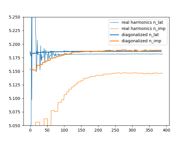
this case). Once the calculation is finished, we examine n_imp and
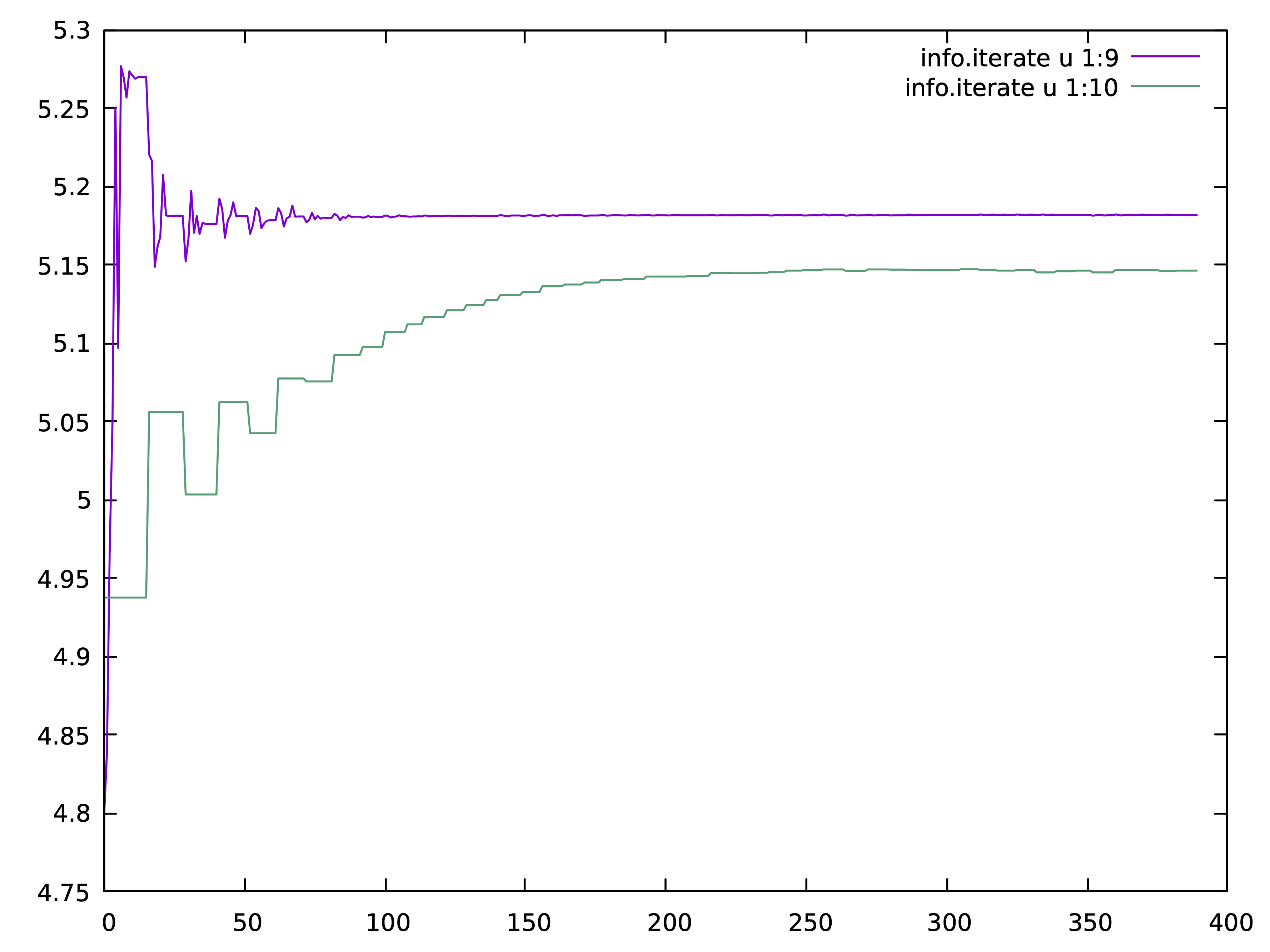
n_latt in info.iterate, i.e., column 9 and 10. If the two values are
sufficiently close, we can be confident in our choice of the
orbitals.
For the RuO2 the current choice of local orbitals is ok, and here is
how it should look like:
 The lattice density is around 5.181 and the impurity density around 5.146,
which is acceptable, but later we will improve that with findRot.py script.
If the values are far off, there is either a bug, or, bad
choice of local orbitals. Currently we use cubic harmonics, but we
can execute "findRot.py" script on resulting calculation if the
mismatch between n_imp and n_latt is too large.
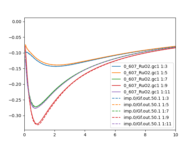
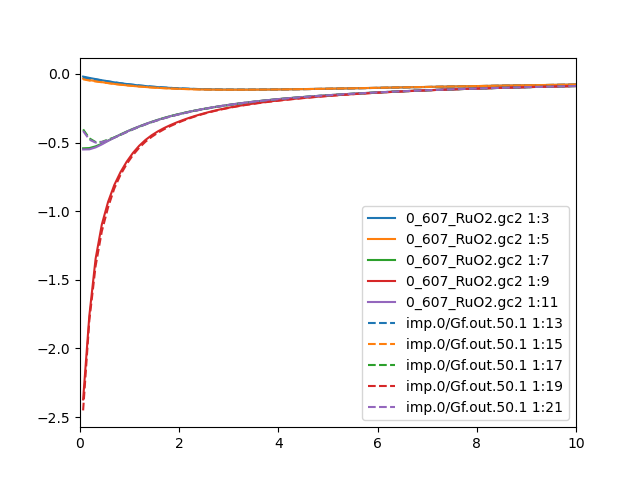
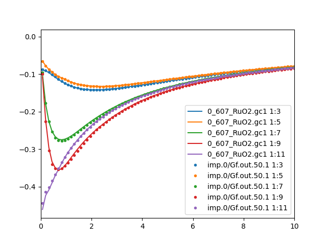
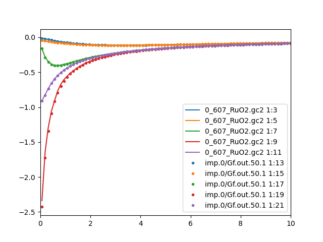
Even better is to compare case.gc[1-2] and imp.0/Gf.out.50.1. This
checks if the local green's function is the same as the impurity
green's function. If green's function is diagonal, our choice of diagonal
hybridization should make these two Green's function equal. But if
hybridization is chosen to be diagonal, while the Green's function is
not, we will have mismatch between the two quantities. Here is how they
look like in this run for up and down spins:

 Similar conclusion can be drawn from the Green's function comparison
than the impurity/lattice density: the agreement is
not perfect, but it is acceptable. Hence we will proceed to the
analytic continuation.
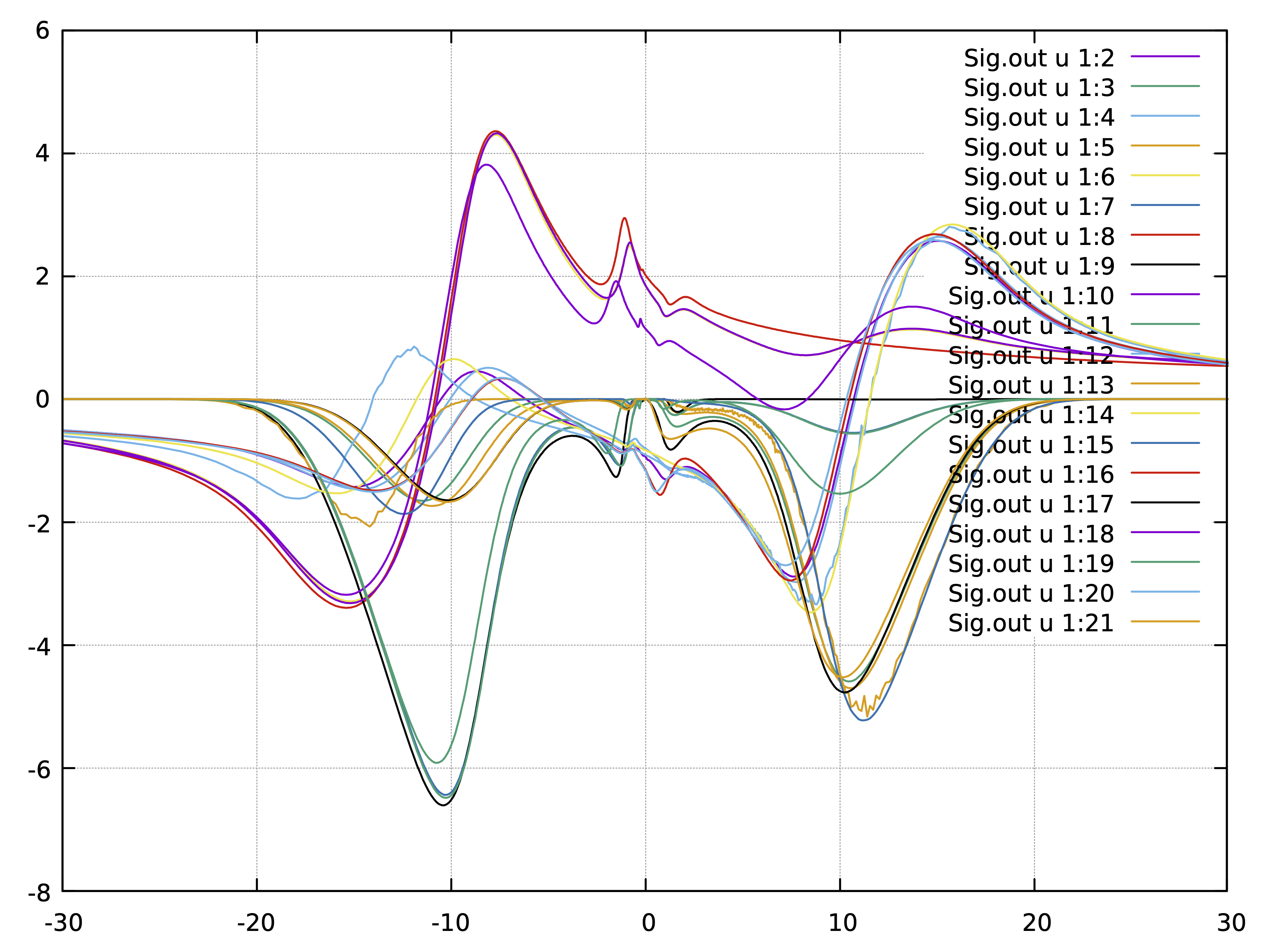
We check a few last eDMFT self-energies (sig.inp.4[5-9].1
sig.inp.50.1) and we confirm that they differ only due to Monte
Carlo noise. We can hence average over the last few iterations. For example:
saverage.py sig.inp.4[5-9] sig.inp.50
For this example we will increase the real axis mesh to 30eV, because
it turns out that in some cases 20eV default is somewhat too small
window on the real axis. We also need to somewhat increase the number
of points on the real axis, since the range has increase (Nw=450). The
rest of the parameters are default, which we used before.
The content of "maxent_params.dat" file should be set to:
params={'statistics': 'fermi', # fermi/bose
        'Ntau'      : 400,     # Number of time points
        'L'         : 30.0,    # cutoff frequency on real axis
        'x0'        : 0.01,    # low energy cut-off
        'bwdth'     : 0.004,   # smoothing width
        'Nw'        : 450,     # number of frequency points on real axis
        'gwidth'    : 2*15.0,  # width of gaussian
        'idg'       : 1,       # error scheme: idg=1 -> sigma=deltag ; idg=0 -> sigma=deltag*G(tau)
        'deltag'    : 0.005,   # error
        'Asteps'    : 4000,    # anealing steps
        'alpha0'    : 1000,    # starting alpha
        'min_ratio' : 0.001,   # condition to finish, what should be the ratio
        'iflat'     : 1,       # iflat=0 : constant model, iflat=1 : gaussian of width gwidth, iflat=2 : input using file model.dat
        'Nitt'      : 1000,    # maximum number of outside iterations
        'Nr'        : 0,       # number of smoothing runs
        'Nf'        : 40,      # to perform inverse Fourier, high frequency limit is computed from the last Nf points
        }

Next we create a directory for the real axis spectra and density of
states. Let's call it "onreal". We enter that subdirectory and copy all necessary files from the
self-consistent run by the script
Here the argument is
the name of the directory with the self-consistent run.
We will compute the band structure on the real axis now. But before we
run eDMFT on k-path in first BZ, we might need to fine tune the path.
The default path is [\Gamma,A,M,R,X,Z] (see "cif2struct.log" or look
into "0_607_RuO2.klist_band"). It turns out that this high symmetry path does not reveal the
nature of altermagnetic band splitting. The splitting is largest
between Gamma-M, hence we will modify the k-path to
[M,\Gamma,M,A,R,X,Z]. To do that, we will execute "klist_gen.py". This
script can be run interactively, or in batch mode. We will use the batch
mode here:
klist_gen.py -n 500 -p "[[0.5,0.5,0],[0,0,0],[0.5,0.5,0],[0.5,0.5,0.5],[0.,0.5,0.5],[0,0.5,0],[0,0,0.5]]" -m "['M','\Gamma','M','A','R','X','Z']"
Now we proceed to calculation of the densities of states and bands. We
execute the following
set of commands in the directory "onreal":
$WIENROOT/x_lapw lapw0 -f 0_607_RuO2 >& nohup.dat
$WIEN_DMFT_ROOT/x_dmft.py lapw1        >& nohup.dat
$WIEN_DMFT_ROOT/x_dmft.py dmft1        >& nohup.dat
$WIEN_DMFT_ROOT/x_dmft.py lapw1 --band >& nohup.dat
$WIEN_DMFT_ROOT/x_dmft.py dmftp        >& nohup.dat
$WIEN_DMFT_ROOT/x_dmft.py dmftp -l dn  >& nohup.dat
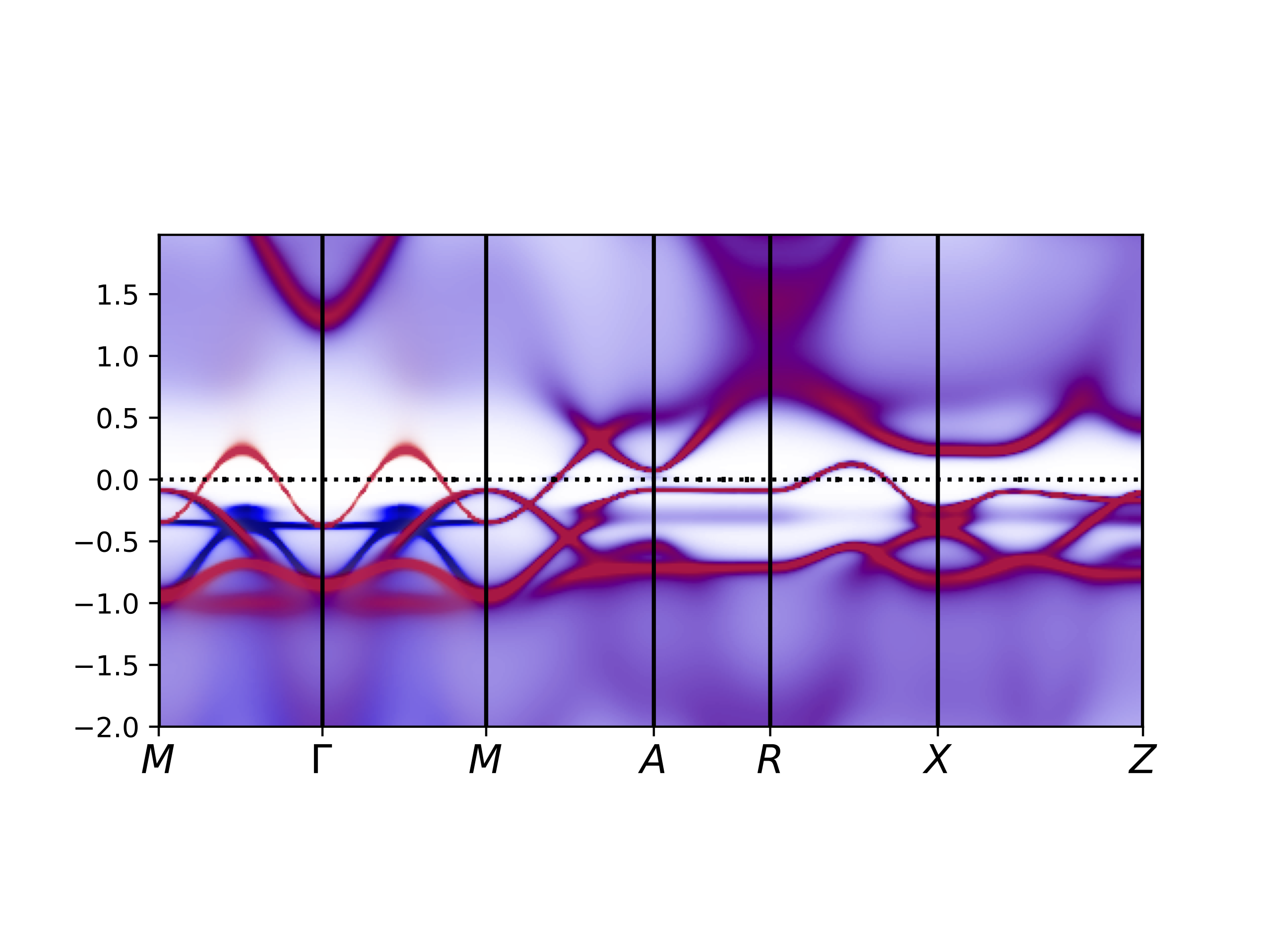
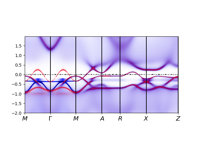
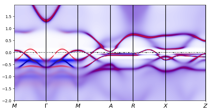
Finally, we want to plot the spectral function of both the up and down
spins simultaneously. We have a dedicated python script for that:
which reads both "eigvals.dat" and "eigvalsdn.dat", and displays them
in red-blue color, respectively.
Here is how it looks like for this run:

The argument for intensity can be given to makplot.py, however, its
value should be between 0-1, and a number very close to 1 is
desired. Default is 0.97.
Namely, in the old version of "wakplot.py" routine we would specify
intensity (the argument) as the ratio between maximum value of Akw
considered when plotting (the cutoff for plotting) and the maximum
value found in the 2D plot. The problem with this algorithm is that
sometimes intensity needs to be reduced to a very small
number. Namely, it sometimes happens that a
very few points (sometimes a single point) in the 2D plot are extremely singular, while
majority of the relevant points have modest values distributed between
[0,v_max]. But v_max in this case is much smaller than the maximum
value we find in 2D plot, hence the ratio (given as input parameter)
must be very small to have a reasonable plot.
In the new version of the plotting program, we obtain the histogram of
values in the 2D plot, and we keep 97\% of the values in the plot,
i.e., 3\% are cut-off for the purpose of the plot. If the shapes
appear too broad and intense, we would increase this number closer to
unity. If the quasiparticle bands appear very faint, we would decrease this value
towards 0.5. But a small value for intensity in this algorithm does
not make much sense.
For this run, the value of
sharpens up the spectra, and produces

Finally, we noticed above that lattice density and impurity density do
not match perfectly at the converged solution, because the impurity
problem is not completely diagonal in our chosen real harmonics
basis. But we have freedom to choose any orbital basis we want, and
a better basis can be often chosen by diagonalizing the hybridization
function at low frequency.
The script "findRot.py" does that. It can diagonalize hybridization
either at low energy, or at infinite frequency, and should
substantially reduce this mismatch.
We will slightly edit the self-energy file and we will add frequency
omega=0 on imaginary axis. This is not essential, but it is a good
idea to diagonalize hybridization at exactly zero frequency, which is
of course equal on real and imaginary axis. We will take the real part
of the self-energy for each orbital from the lowest matsubara point,
while we will zero out imaginary parts (because they should vanish at
zero frequency in a metal). The first two lines of the data in the
"sig.inp" file look like that
0.0                      -9.299057493961586651e-01  0.0                      -7.980767955268603941e-01   0.0                     1.856077099430119670e+00 0 ....
6.283185307179600665e-02 -9.299057493961586651e-01 -2.480501738282099924e-02 -7.980767955268603941e-01 -1.601768961148599887e-02 1.856077099430119670e+00 -3.745090133373799729e-02 ...
x_dmft.py  lapw1
x_dmft.py  dmft1
 omega~0 is  0.000000000000000E+000 at i=           1
 Full matrix of impurity levels follows
 icix=           1
   -2.19442993    -0.00000000       0.02491185    -0.00000000       0.00001048    -0.00000000      -0.10556106     0.00000000      -0.00000777     0.00000000
    0.02491185     0.00000000      -2.22316952    -0.00000000      -0.00001503     0.00000000       0.18283159    -0.00000000       0.00001659    -0.00000000
    0.00001048     0.00000000      -0.00001503    -0.00000000      -4.07898996    -0.00000000       0.00000261     0.00000000       0.03014284    -0.00000000
   -0.10556106    -0.00000000       0.18283159     0.00000000       0.00000261    -0.00000000      -3.83831649     0.00000000      -0.00000261    -0.00000000
   -0.00000777    -0.00000000       0.00001659     0.00000000       0.03014284     0.00000000      -0.00000261     0.00000000      -4.07898793     0.00000000

 icix=           1 at omega=0
    2.30955442    -0.00000000      -1.99477879     0.00000000      -0.00013691     0.00000000      -0.42448657     0.00000000       0.00015658     0.00000000
   -1.99477879    -0.00000000       4.60893257    -0.00000000       0.00030171     0.00000000       0.73482339     0.00000000      -0.00020871    -0.00000000
   -0.00013691    -0.00000000       0.00030171    -0.00000000      -3.46926140    -0.00000000      -0.00029553     0.00000000       0.24824833    -0.00000000
   -0.42448657    -0.00000000       0.73482339    -0.00000000      -0.00029553    -0.00000000      -3.50311324     0.00000000       0.00029820    -0.00000000
    0.00015658    -0.00000000      -0.00020871     0.00000000       0.24824833     0.00000000       0.00029820     0.00000000      -3.46903791     0.00000000

 icix=           2
   -2.19530225    -0.00000000       0.02477157    -0.00000000       0.00000775    -0.00000000      -0.10494473    -0.00000000      -0.00000479     0.00000000
    0.02477157     0.00000000      -2.22386664     0.00000000      -0.00001001     0.00000000       0.18176118     0.00000000       0.00001172     0.00000000
    0.00000775     0.00000000      -0.00001001    -0.00000000      -4.07979893     0.00000000       0.00000060     0.00000000       0.03043344     0.00000000
   -0.10494473     0.00000000       0.18176118    -0.00000000       0.00000060    -0.00000000      -3.83803086    -0.00000000      -0.00000060     0.00000000
   -0.00000479    -0.00000000       0.00001172    -0.00000000       0.03043344     0.00000000      -0.00000060    -0.00000000      -4.07979861     0.00000000

 icix=           2 at omega=0
    3.09647612    -0.00000000      -1.48434905     0.00000000       0.00087385    -0.00000000      -0.00526244    -0.00000000      -0.00005241     0.00000000
   -1.48434905    -0.00000000       4.82431354     0.00000000      -0.00055118     0.00000000       0.01001850    -0.00000000       0.00100097    -0.00000000
    0.00087385     0.00000000      -0.00055118    -0.00000000      -2.91196068     0.00000000       0.00005605     0.00000000       0.49142684    -0.00000000
   -0.00526244     0.00000000       0.01001850     0.00000000       0.00005605    -0.00000000      -3.44759215    -0.00000000      -0.00004601    -0.00000000
   -0.00005241    -0.00000000       0.00100097     0.00000000       0.49142684     0.00000000      -0.00004601     0.00000000      -2.91328536     0.00000000
The script also corrected "0_607_RuO2.indmfl" file, which now has the
following local orbitals on Ru[0]
 0.35378068  0.00000504    0.00000522  0.00001678    0.86583974  0.00000000   -0.00000522  0.00001678    0.35378068 -0.00000504
-0.60972979  0.00001695   -0.00002246 -0.06397079    0.49827165  0.00000000    0.00002246 -0.06397079   -0.60972979 -0.00001695
 0.00020813  0.49988468   -0.50010977 -0.00233687   -0.00016978  0.00000000    0.50010977 -0.00233687    0.00020813 -0.49988468
 0.05539642 -0.00166417    0.00165785 -0.70420329   -0.04524249  0.00000000   -0.00165785 -0.70420329    0.05539642  0.00166417
 0.00000660 -0.50011252   -0.49988745  0.00000533    0.00000647  0.00000000    0.49988745  0.00000533    0.00000660  0.50011252
 0.35248283  0.00006914    0.00007282  0.00005369    0.86689773  0.00000000   -0.00007282  0.00005369    0.35248283 -0.00006914
-0.61298876 -0.00006949    0.00007121 -0.00087625    0.49848571  0.00000000   -0.00007121 -0.00087625   -0.61298876  0.00006949
 0.00004893 -0.49966294   -0.50033683 -0.00000490    0.00012396  0.00000000    0.50033683 -0.00000490    0.00004893  0.49966294
-0.00078652  0.00084366   -0.00084945  0.70710522    0.00055202 -0.00000000    0.00084945  0.70710522   -0.00078652 -0.00084366
 0.00008365 -0.50033611    0.49966221  0.00119733   -0.00007231 -0.00000000   -0.49966221  0.00119733    0.00008365  0.50033611
Next we want to rerun dmft1 step, and check how diagonal are impurity
levels now:
The output in "0_607_RuO2.outputdmf1" is
 omega~0 is  0.000000000000000E+000 at i=           1
 Full matrix of impurity levels follows
 icix=           1
   -2.18004748     0.00000000       0.00001289     0.00000000       0.00000022    -0.00000000      -0.00004107     0.00000000       0.00001917    -0.00000000
    0.00001289    -0.00000000      -2.21263596    -0.00000000       0.00013626    -0.00000000       0.06353508    -0.00000000      -0.00001056     0.00000000
    0.00000022     0.00000000       0.00013626     0.00000000      -4.10911936     0.00000000       0.00081448     0.00000000       0.00001455     0.00000000
   -0.00004107    -0.00000000       0.06353508     0.00000000       0.00081448    -0.00000000      -3.86331357     0.00000000      -0.00000171     0.00000000
    0.00001917     0.00000000      -0.00001056    -0.00000000       0.00001455    -0.00000000      -0.00000171    -0.00000000      -4.04884784     0.00000000

 icix=           1 at omega=0
    1.06866021     0.00000000      -0.00490263    -0.00000000       0.00000106    -0.00000000      -0.00014357    -0.00000000       0.00004811     0.00000000
   -0.00490263     0.00000000       5.82362525    -0.00000000      -0.00039349     0.00000000      -0.00137855     0.00000000      -0.00004948     0.00000000
    0.00000106     0.00000000      -0.00039349    -0.00000000      -3.71341613     0.00000000       0.00045141     0.00000000       0.00015137    -0.00000000
   -0.00014357     0.00000000      -0.00137855    -0.00000000       0.00045141    -0.00000000      -3.58091974     0.00000000       0.00000151     0.00000000
    0.00004811    -0.00000000      -0.00004948    -0.00000000       0.00015137     0.00000000       0.00000151    -0.00000000      -3.21766437     0.00000000

 icix=           2
   -2.18104942    -0.00000000      -0.00011523     0.00000000       0.00026524    -0.00000000      -0.00049293    -0.00000000      -0.00000774     0.00000000
   -0.00011523    -0.00000000      -2.23759918     0.00000000       0.00000472     0.00000000      -0.20796699     0.00000000      -0.00061574     0.00000000
    0.00026524     0.00000000       0.00000472    -0.00000000      -4.04936646    -0.00000000      -0.00000197    -0.00000000       0.00004117     0.00000000
   -0.00049293    -0.00000000      -0.20796699     0.00000000      -0.00000197     0.00000000      -3.83847698    -0.00000000       0.00048766    -0.00000000
   -0.00000774    -0.00000000      -0.00061574    -0.00000000       0.00004117    -0.00000000       0.00048766     0.00000000      -4.11017740     0.00000000

 icix=           2 at omega=0
    2.24446045    -0.00000000       0.00586448     0.00000000       0.00084256    -0.00000000      -0.00046833    -0.00000000      -0.00002755     0.00000000
    0.00586448    -0.00000000       5.62743693     0.00000000       0.00001635     0.00000000      -0.00372699    -0.00000000      -0.00449864     0.00000000
    0.00084256     0.00000000       0.00001635    -0.00000000      -2.41907272    -0.00000000       0.00000532    -0.00000000       0.00062370    -0.00000000
   -0.00046833     0.00000000      -0.00372699     0.00000000       0.00000532     0.00000000      -3.44784432    -0.00000000      -0.00055677    -0.00000000
   -0.00002755    -0.00000000      -0.00449864    -0.00000000       0.00062370     0.00000000      -0.00055677     0.00000000      -3.39060635     0.00000000
One more word of caution is in order. The current script "findRot.py"
currently changes only case.indmfl but not case.indmfldn. Once we are
happy with the choice of the orbitals in case.indmfl, we should also
change orbitals in case.indmfldn accordingly. For example, orbitals
1-5 in case.indmfl should be copied to 6-10 in case.indmfldn, and
viceversa.
Once we updated "0_607_RuO2.indmfl" and "0_607_RuO2.indmfldn", we copy
them to the converged run, and resubmit the job, to converge it again
with this superior choice of orbitals. The difference between the
impurity and lattice density disappears, and info.iterate (column 9
and 10) show the following:
 We included for reference the original run with real harmonics, which
is compared with this run using diagonalized local orbitals.
The Green's function mismatch is also eliminated. We plot the
comparison between the impurity and lattice Green's function for
both Ru sites:


We now repeat previous steps to obtain the real axis spectra:
saverage.py sig.inp.4[5-9] sig.inp.50
mkdir maxent
cd maxent
cp ../sig.inpx .
cp ../../oldrun/maxent/maxent_params.dat .
maxent_run.py sig.inpx
mkdir ../onreal
cd ../onreal
dmft_copy.py ../
cp ../../oldrun/onreal/0_607_RuO2.klist_band
x_lapw lapw0 -f 0_607_RuO2
x_dmft.py lapw1 --band
x_dmft.py dmftp
x_dmft.py dmftp -l dn
makplot.py 0.99

Plotting 2D cuts of spectral function at EF
In this section we will plot the Fermi surface as a 2D cut in the
BZ. This will show if the system has particular symmetry at the Gamma
point, i.e., d-wave symmetry, for example.
To do that, we first prepare input file "2D_params.py" in which we
write 2D path we want to take in first BZ. The file can contain a
single line, like:
This means that we will make a cut at z=0. We choose the variable x to
go from [-1,1], and variable y to also go from [-1,1]. Using these two
variables, we define 2D plane in BZ for the 2D plot.
We can execute
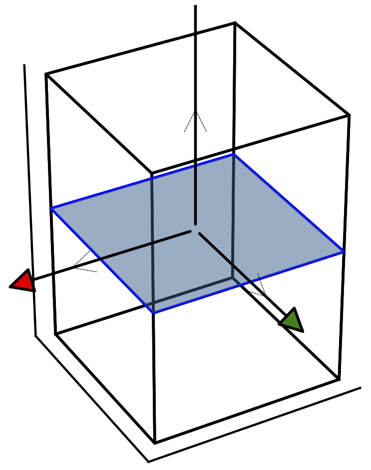
which will plot the first Brillouin zone and the 2D cut we choose to
make.
 The python script bz.py will produce the plot of the BZ.
The blue plane shows the 2D cut we are making. The thick arrows are
three reciprocal basis vectors, and the thin lines are chosen
cartesian basis vectors. Note that the 2D plane in kpath=[] should be
specified in cartesian basis, which is usually easier to comprehend
than reciprocal basis. Note that the latter is in general
non-orthogonal, while cartesian basis is always orthonormal. In this
simple case the two basis coincide. Note also that
red/gren/blue arrows stand for x/y/z direction.
Next we execute
which will produce "case.klist_band" that can be used to plot
spectra. By default the number of k-points in single direction is
"Nxy=90", which can be changed, if desired. Number of all k-points for
this 2D plot is 91^2=8281. But when case.struct file contains all
symmetry operations, this number can be reduced substantially. For
example, RuO2 has 8 symmetry operations, and the non-equivalent
momentum points are cut down to 2116.
The output should say something like
Number of all irreducible points= 2116 versus all= 8281
0 0.025 0.025 2 0.0 0.01 # matsubara, broadening-corr, broadening-noncorr, nomega, omega_min, omega_max (in eV)
x_dmft.py lapw1 --band
x_dmft.py dmftp
x_dmft.py dmftp -l dn
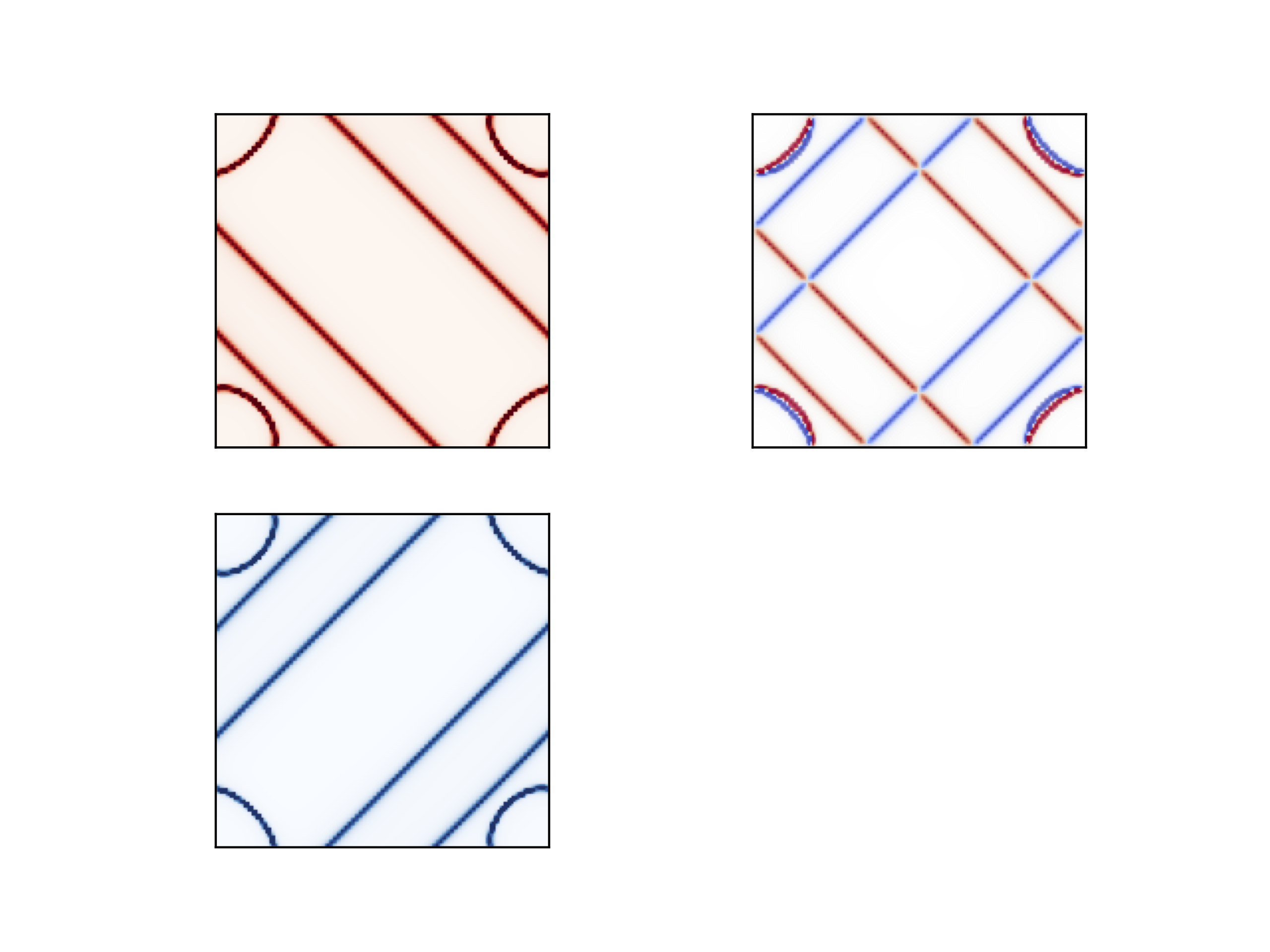
 On the left we see separately
Fermi surface for up and down spins. On the right we see the combined
plot with both spins present. Clearly the cut shows d-wave symmetry.
Last modified: Sat Dec 28 14:12:57 EST 2024
