Home What is? Install Overview CTQMC MnO FeSe SrVO3 LaVO3 Cerium Sr2IrO4 Ta2NiSe5 phonon

Tutorial 1: MnO

Tutorial 1.a. : Preparing the input files

We begin by a simple example of a charge transfer insulator: MnO. It cristalizes in the rock salt structure (two interpenetrating cubic FCC str.) with lattice parameter 8.401155a a.u.. The Mn ion contains around 5 electrons, which form the high spin state. The ground state has a large gap, which is usually categorized as the charge transfer gap. We will treat dynamically the Mn-d electrons.

The first step is to perform a DFT calculation to get a good charge density. (We assume that the user has some familiarity with the Wien2K code and we give only a very brief introductions to the DFT part.)

First create a directory with the name MnO and copy the MnO.struct file into it. [Note that Wien2k requires to call directory with the same name as the structure file]. The structure file contains the details of the crystal structure in the format that Wien2K uses. Initialize the DFT calculation by using init_lapw and then choosing the default options. In version 14, one needs to type the following sequence of commands:

Enter reduction in %:   0
Use old or new scheme (o/N) : N
Do you want to accept these radii; .... (a/d/r) : a
specify nn-bondlength factor: 2
Ctrl-X-C
continue with sgroup : c
Ctrl-X-C
continue with symmetry : c
Ctrl-X-C
continue with lstart : c
specify switches for instgen_lapw (or press ENTER): ENTER
SELECT XCPOT: 13
SELECT ENERGY : -6
Ctrl-X-C
continue with kgen : c
Ctrl-X-C
Ctrl-X-C
NUMBER OF K-POINTS : 500
Ctrl-X-C
continue with dstart or execute kgen again or exit (c/e/x) : c
Ctrl-X-C
do you want to perform a spinpolarized calculation : n

Here Ctrl-X-C stands for breaking out of your editor. Ctrl-XC is used in emacs and similar editors, but in vi, one should replace Ctrl-X-C by :q!.

These are pretty much the default values that Wien2K uses. We chose to work with the PBE functional (note that total energies are better with LDA+DMFT functional, while spectra is almost identical when using PBE or LDA), and use a k-point grid of 500 points (in the whole Brillouin zone). Note that spin-orbit interaction can be safely ignored as there are no heavy ions in the system.

Note that instead of using the interactive way of determining the DFT parameters, one can run wien2k initialization in batch mode, by executing init_lapw with parameters:

init_lapw -b -vxc 13 -ecut -6.0 -rkmax 7 -numk 500

Next, we can run the DFT calculation using the command

run_lapw

In DMFT calculation, one needs converged frequency dependent local Green's function, hence more k-points are typically needed. We will increase the number of k-points to 2000 in this tutorial. To do that, run

x kgen

and specify 2000 k-points. Next, rerun wien2k on this k-mesh, i.e.,

run_lapw -NI

(This step is not essential as the DFT charge will not be very precise anyway for our DFT+Embedded-DMFT calculation).

Once the DFT calculation is done, we have a good charge density to start a DMFT calculation. The next step is to initialize the DMFT calculation. For this, we use the script init_dmft.py. Note that we can execute this python script interactively, or, with giving parameters to the executable (batch mode).
Using faster batch mode, we might want to initialize dmft by

init_dmft.py -ca 1 -ot d -qs 7

The switch -ca specifies the correlated atom, -ot specifies the orbital type, and -qs specifies the cubic symmetry that we are going to use for this orbitals. These options are explained below.

Alternatively, we might want to use the script init_dmft.py in interactive mode, in which case we just execute it, and answer the following questions:

Specify correlated atoms (ex: 1-4,7,8):  1

Do you want to continue; or edit again? (c/e): c

For each atom, specify correlated orbital(s) (ex: d,f):
  1 Mn: d

Do you want to continue; or edit again? (c/e): c

Specify qsplit for each correlated orbital (default = 0):
  1  Mn-1 d: 7

Do you want to continue; or edit again? (c/e): c

Specify projector type (default = 5): 5

Do you want to continue; or edit again? (c/e): c

Do you want to group any of these orbitals into cluster-DMFT problems? (y/n): n

Enter the correlated problems forming each unique correlated
problem, separated by spaces (ex: 1,3 2,4 5-8): 1

Do you want to continue; or edit again? (c/e): c

Range (in eV) of hybridization taken into account in impurity
problems; default -10.0, 10.0: <ENTER>

Perform calculation on real; or imaginary axis? (i/r) (default=i) : i

Ctrl-X-C

Is this a spin-orbit run? (y/n): n

Ctrl-X-C

Now we want to explain the options and their choice:

At the beginning, the code shows all atoms in the unit cell:
There are 2 atoms in the unit cell: 1 Mn 2 O Specify correlated atoms (ex: 1-4,7,8): 1
and asks which one should be treated dynamically. We choose only the first atom, Mn, to be treated as a correlated atom in the DMFT step.
The code next asks which orbital quantum numbers should be treated dynamically:
For each atom, specify correlated orbital(s) (ex: d,f): 1 Mn: d
The partially filled d shell of the Mn ion is to be treated in DMFT.

Next we should specify what type of local symmetry we have on the given atom, and if we possibly want to correlated only a sub-shell

Specify qsplit for each correlated orbital (default = 0): Qsplit Description ------ ------------------------------------------------------------ 0 average GF, non-correlated 1 |j,mj> basis, no symmetry, except time reversal (-jz=jz) -1 |j,mj> basis, no symmetry, not even time reversal (-jz=jz) 2 real harmonics basis, no symmetry, except spin (up=dn) -2 real harmonics basis, no symmetry, not even spin (up=dn) 3 t2g orbitals -3 eg orbitals 4 |j,mj>, only l-1/2 and l+1/2 5 axial symmetry in real harmonics 6 hexagonal symmetry in real harmonics 7 cubic symmetry in real harmonics 8 axial symmetry in real harmonics, up different than down 9 hexagonal symmetry in real harmonics, up different than down 10 cubic symmetry in real harmonics, up different then down 11 |j,mj> basis, non-zero off diagonal elements 12 real harmonics, non-zero off diagonal elements 13 J_eff=1/2 basis for 5d ions, non-magnetic with symmetry 14 J_eff=1/2 basis for 5d ions, no symmetry ------ ------------------------------------------------------------ 1 Mn-1 d: 7

This chooses the local basis for the DMFT calculation. Notice that current implementation of the DMFT in combination with CTQMC is basis dependent. This is because by default we ignore off-diagonal components of the hybridization function. (The code also supports off-diagonal hybridization, but its use requires more advanced options, and leads to a minus sign problem in the solution of the impurity.)
In MnO, we ignored the spin-orbit coupling, and the crystal symmetry is cubic, hence hybridization is exactly diagonal in the cubic harmonics basis. We thus want to use this basis, which is the option 7. We could also use option 2, but this would lead to a slight worse statistics as impurity solver now averages over 3 t2g (or 2 eg) equivalent orbitals.

Specify projector type (default = 5): Projector Drscription ------ ------------------------------------------------------------ 1 projection to the solution of Dirac equation (to the head) 2 projection to the Dirac solution, its energy derivative, LO orbital, as described by P2 in PRB 81, 195107 (2010) 4 similar to projector-2, but takes fixed number of bands in some energy range, even when chemical potential and MT-zero moves (folows band with certain index) 5 fixed projector, which is written to projectorw.dat. You can generate projectorw.dat with the tool wavef.py ------ ------------------------------------------------------------ > 5
As discussed above, DMFT requires a local basis, i.e., projector to local Green's function. If we could treat by DMFT all degrees of freedom on a given atom, the solution would not depend on the choice of the projector (it would depend on the range though). Fortunately, the orbitals on Mn ion are quite nicely separated in energy, and the only narrow states close to EF on Mn ion are the 3d states, hence they become correlated. Note that the Mn 4s orbital is not far above EF, but the 4s state is very spatially extended, hence weakly correlated.
All choices of the projector project to spherical/cubic harmonics inside a sphere around an atom, but the radial dependence of the function is slightly different. "Projector 1" chooses solution of the Dirac equation for the radial part, "Projector 2" chooses a combination of the Dirac equation solution and its energy derivative, "Projector 4" has the same radial component as Projector 2, but when choosing an energy range for the projector, it will use equal number of bands at each k-point (projector will follow bands). Finally, projector 5 fixes the projector to the solution of the Dirac equation on the LDA level.
If we are interested in the total free energy of the system, we should use projector 5, because in this case the projector is fixed during DMFT self-consistent run, which guarantees that the DFT+Embedded-DMFT method is stationary.
Cluster versus single-site DMFT option:

Do you want to group any of these orbitals into cluster-DMFT problems? (y/n): n

We do not attempt to do a cluster-DMFT calculation at this stage.
For efficiency reasons, we want to solve impurity only for those atoms which are different (and not related by symmetry). While we could figure this out from the structure file, we allow the user to set this here independently of the symmetry in the structure file. This allows one to treat spontaneously broken states (such as magnetically ordered states) in DMFT without reducing the crystal symmetry.

Enter the correlated problems forming each unique correlated problem, separated by spaces (ex: 1,3 2,4 5-8): 1

There is only one impurity in this system anyway.
Choice for the energy range in the Kohn-Sham basis
Range (in eV) of hybridization taken into account in impurity problems; default -10.0, 10.0:
This sets the energy range around the Fermi level, where the hybridizations will be taken into account. Usually a value of the order of U is a good starting guess, but one should check the resultant hybridization to see that it is enough. "Projector 1" and "Projector 2" will use all bands in this energy range. "Projector 4" and "5" will use the same set of bands at each k-point, and to faithfully represent the states in this energy range, it will automatically increase the energy range in some k-points.

Perform calculation on real; or imaginary axis? (r/i): i

The CTQMC is an imaginary axis method.

Is this a spin-orbit run? (y/n): n
The spin-orbit coupling is ignored.

The init_dmft.py script generates two mandatory input files, case.indmfl and case.indmfi, and also projectorw.dat when fixed projector=5 is used. These files connect the solid and the impurity with the DMFT engine, respectively. Let us take a closer look at the header of the case.indmfl file:

5 15 1 5                              # hybridization band index nemin and nemax, renormalize for interstitials, projection type
1 0.025 0.025 200 -3.000000 1.000000  # matsubara, broadening-corr, broadening-noncorr, nomega, omega_min, omega_max (in eV)
1                                     # number of correlated atoms
1     1   0                           # iatom, nL, locrot
  2   7   1                           # L, qsplit, cix

The first line specifies the hybridization window. We set it to "(-10eV,10eV)" around EF, which it turns out, contains bands numbered from 5-15. For each k-point we will use the same bands, i.e., we will follow the bands with the projector.
The same line also specified the projector type, which is 5.
The second line contains a switch for the real-axis or imaginary axis calculation. If we require the local green's function or density of states on real axis, we will set the switch "matsubara" to 0. Here, we will work on imaginary axis, hence "matsubara" is set to 1. The second line also contains information on small lorentzian broadening in k-point summation. The last three numbers are used for plotting the spectral functions, to which we will return latter.
The third line specifies the number of correlated atoms.
The forth line specifies which atom (from case.struct) is correlated (Note that each atom in the structure file counts, even when several atoms in structure files are equivalent). The forth line also specifies how many orbital indeces (different L's) we will use for projection, and calculation of local green's function and partial dos. The last index "locrot" is used for rotation of local axis, and is not needed here (set to 0).
The fifth line specifies orbital momentum "l=2", "qsplit=7" which we chose during initialization. Each correlated orbital-set gets a unique index during initialization. This correlated set was given index "cix=1". For each correlated set, a more detailed specification is needed, which is given in the remaining of "case.indmfl" file.

The specification of correlated set is given in the second part of case.indmfl:

#================ # Siginds and crystal-field transformations for correlated orbitals ================
1     5   2       # Number of independent kcix blocks, max dimension, max num-independent-components
1     5   2       # cix-num, dimension, num-independent-components
#---------------- # Independent components are --------------
'eg' 't2g' 
#---------------- # Sigind follows --------------------------
1 0 0 0 0
0 1 0 0 0
0 0 2 0 0
0 0 0 2 0
0 0 0 0 2
#---------------- # Transformation matrix follows -----------
 0.00000000 0.00000000   0.00000000 0.00000000   1.00000000 0.00000000   0.00000000 0.00000000   0.00000000 0.00000000 
 0.70710679 0.00000000   0.00000000 0.00000000   0.00000000 0.00000000   0.00000000 0.00000000   0.70710679 0.00000000 
 0.00000000 0.00000000   0.70710679 0.00000000   0.00000000 0.00000000  -0.70710679 0.00000000   0.00000000 0.00000000 
 0.00000000 0.00000000   0.00000000 0.70710679   0.00000000 0.00000000   0.00000000 0.70710679   0.00000000 0.00000000 
-0.70710679 0.00000000   0.00000000 0.00000000   0.00000000 0.00000000   0.00000000 0.00000000   0.70710679 0.00000000

The first line specifies the number of all correlated blocks, the dimension of the largest correlated block, and number of orbital components which differ. The second line specifies the dimension of the first correlated block (here "d" has dimension 5), and the two eg and the three t2g components are treated as degenerate.

The transformation matrix from spheric harmonics to the DMFT basis is given in the end, and shows how these orbitals are defined: It is the expansion of each of these orbitals in spherical harmonics. The columns correspond to the following quantum numbers (m_l=-2,-1,0,1,2) and rows to ('z^2','x^2-y^2','xz','yz','xy'). For example, the 'z^2' orbital, which is expanded in the first line, is equal to the m=0 spherical harmonic, whereas the yz orbital on the forth line is an equal superposition of m=1 and m=-1, multiplied by i (note that two consecutive real numbers define one complex number). Note that the transformation matrix must be unitary.

This file case.indmfl can be edited in text editor and can be adjusted if necessary.

The second file, created at the initialization, is case.indmfi and contains the following lines:

1   # number of sigind blocks
5   # dimension of this sigind block
1 0 0 0 0
0 1 0 0 0
0 0 2 0 0
0 0 0 2 0
0 0 0 0 2

In this simplest case, where we have a single impurity problem, no new information is contained in case.indmfi file, just the "Sigind" block from case.indmfl is repeated. We will show more complex use of this file later.

Now we want to start DMFT with the minimal number of necessary files. To do this, create a new folder (with any name), and when in that folder, use the command

dmft_copy.py <dft_results_directory>

where <dft_results_directory> is the directory where the output of the DFT calculation with DMFT initialization is. This command copies the necessary files to start a DMFT calculation. These include the MnO.struct file as well as the various Wien2K input files such as MnO.inm, MnO.in1, etc. The charge density file, MnO.clmsum, is also copied. This is all we need from the initial Wien2K run, and now we proceed to create the rest of the files, needed by the DMFT calculation.

Copy the params.dat file. This file contains information about the impurity solver and additional parameteres, which appear in DFT+Embedded-DMFT. It is written in Python format, and hence any Python syntax is accepted. For checking the correct syntax, one can execute it as python script. Its content is:

solver         =  'CTQMC'   # impurity solver

max_dmft_iterations = 1     # number of iteration of the dmft-loop only
max_lda_iterations  = 100   # number of iteration of the LDA-loop only
finish              = 10    # number of iterations of full charge loop  (1 = no charge self-consistency).
                            # You should probably  use 30 or so, but for testing 10 is OK.

ntail          =  300       # on imaginary axis, number of points in the tail of the logarithmic mesh

cc             =  5e-6      # the charge density precision to stop the LDA+DMFT run
ec             =  5e-6      # the energy precision to stop the LDA+DMFT run
recomputeEF    =  0         # Recompute EF in dmft2 step. If recomputeEF = 0, EF is fixed. Good for insulators.

DCs            =  'exactd'  # exact DC with dielectric model  

wbroad         =  0.0       # broadening of sigma on the imaginary axis
kbroad         =  0.0       # broadening of sigma on the imaginary axis

# Impurity problem number 0
iparams0={"exe"                : ["ctqmc"               , "# Name of the executable"],
          "U"                  : [9.0                   , "# Coulomb repulsion (F0)"],
          "J"                  : [1.14                  , "# Coulomb J"],
          "CoulombF"           : ["'Ising'"             , "# Density-density form. Can be changed to 'Full' "],
          "beta"               : [38.68                 , "# Inverse temperature"],
          "svd_lmax"           : [25                    , "# We will use SVD basis to expand G, with this cutoff"],
          "M"                  : [5e6                   , "# Total number of Monte Carlo steps per core"],
          "mode"               : ["SH"                  , "# We will use Greens function sampling, and Hubbard I tail"],
          "nom"                : [100                   , "# Number of Matsubara frequency points sampled"],
          "tsample"            : [30                    , "# How often to record measurements"],
          "GlobalFlip"         : [500000                , "# How often to try a global flip"],
          "warmup"             : [1e5                   , "# Warmup number of QMC steps"],
          "nf0"                : [5.0                   , "# Nominal valence we expect. Used only for starting DC."],
          }

Note that this input file is a python script, and the correcteness of its syntax can be checked with Python interpreter by tying python params.dat. Below we explain the meaning of the variables

```
solver = 'CTQMC'
```
The impurity solver to be used in the calculation. CTQMC stands for Continous Time Quantum Monte Carlo. Only this solver will be used in these tutorials. Alternative solver is 'OCA' (one crossing approximation).
```
max_dmft_iterations = 1
```
First recall the global computational scheme from the introduction:

There is the dmft loop in red, the DFT loop in grey, and the global loop that connects both loops. This variable sets the maximum number of steps inside the dmft (ref) loop. As we set the variable to 1, a single DMFT step (solution of the impurity problem) will be performed every time the global loop is executed. In this example the impurity solver is much slower than the DFT part, hence we will solve the impurity problem only once inside the charge DFT+Embedded-DMFT loop.
```
max_lda_iterations = 100
```
After each DMFT step (impurity solver), the code performs up-to 100 DFT steps (the grey loop in figure). Once we are close to the solution, the charge will converge must faster than in 100 steps, hence we will completely converge charge at each self-energy update. Notice that broyden is very efficiently used here (when self-energy is fixed).
```
finish         =  30
```
Maximum total number of DFT+Embedde-DMFT global steps, each of which include single DMFT step and up to 100 DFT steps.
```
ntail         =  300
```
The self-energy on imaginary axis contains very many Matsubara points (20,000 is quite common), hence we do not want to compute hybridization function for all these points. Fortunately, high frequency tail on imaginary axis contains very little information, hence it can be very well described by a logarithmic mesh of Matsubara points. In computing hybridization function and charge density, we compute first "nom" points exactly, and the rest are approximated with ntail=300 logarithmically distributed Matsubara points. Internally, we either use spline or second order interpolation, to get functions on all Matsubara points.
```
cc             =  5e-6      # the charge density precision to stop the LDA+DMFT run
ec             =  5e-6      # the energy precision to stop the LDA+DMFT run
```
The DFT loop will stop after it reaches the above given limit (max_lda_iterations). The loop will also stop when both the charge and energy are sufficiently converged (difference of charge less than cc, and energy less then ec).
```
recomputeEF = 0
```
The chemical potential will not be re-calculated at each step. For metals, we should always re-calculate the chemical potential. For Mott insulators, the continuous update of the chemical potential does not work well, because the position of the Fermi level is not well defined and its position will jump inside the gap (due to numerics).

One way is to first switch on the search for the chemical potential (recomputeEF=1), and then monitor the progress of the calculation. Once it starts jumping inside the gap, one can fix it roughly into the middle of the gap, to allow nice convergence of the DMFT loop. There are several ways to estimate what is the "middle of the gap". Maybe the easiest is to look at the impurity Green's function (imp.0/Gf.out.?.1). When the gap opens, the imaginary part of G (for all orbitals) will go to zero at zero frequency. The real part of G will be small when G appears roughly particle-hole symmetric at low energy, which means that chemical potential is roughly in the middle of the gap. When we see that for some iterations Im(G(0))=0 and Re(G(0)) small, we should look into info.iterate what was the chemical potential at that step, and set this value into EF.dat.

Far more simple way is to just fix the chemical potential to the LDA value (fix it at the very beginning of the run), and than wait to see if the gap in the Green's function develops after a few iterations. If it does, the chemical potential is most likely in the gap. To make sure that this is not a "fake" gap, we need to scroll to the end of dmft2_info.out, and check the line which says someting like:
```
Ratio to renormalize= 1.000120921355 rho-rho_expected=  -0.0022972280
```
The same information is also printed in MnO.scf file with the key-word :DRHO, hence
```
grep ':DRHO' MnO.scf
```
will print the entire history of charge mismatch. This number shows that the charge density is very close to what we expected. Currently it has 2.3e-3 electron missing, which is definitely due to finite precision in computing the electronic charge. Notice that if we hit a "fake" gap, the charge density will be wrong for an integer number, i.e., "rho-rho_expected" will be close to +1.0 or -1.. Note also that at the first few iterations the density might not be so precise and "rho-rho_expected" might be finite. But once the Green's function stops changing, the density should be correct.
```
DCs            =  'exactd'  # exact double-counting with dielectric constant 
```
The double counting scheme (DCs): In this calculation we are using the exact double-counting assuming dielectric screening.

There are several possible choices for the double-counting.
- The most stable is the nominal choice
  DCs='nominal'
  in which case we need to specify the expected nominal occupancy of the ionic state. This is done through parameter nf0 in iparams0 (see below). We then evaluate
  
  As explained in PRL 115, 196403, this choice is quite close to the exact DC, which we explain below.
- For many metallic systems the Yukawa form of the screening is quite good, i.e.,
  DCs='exacty'
  which means that in real space, the DMFT Coulomb repulsion is assumed to have the form
  and the screening length is determined such that
- In some insulators, the dielectric screening is better, which can be used by selecting the option
  DCs='exactd'
  which assumes
- Most often the best choice is somewhere between the two described options (yukawa and dielectric), and we implemented a combination of the two, which we call
  DCs='exact'
  and assumes the form
  Of course, the equation still needs to be satisfied.
- We also allow the so-called fully-localized-limit
  DCs='FLL'
  double-counting, but we do not recommend it.
Note that in MnO the results of exactd, nominal and exact double-countings are similar, for example converged nd=5.03 with exactd and nd=4.97 with exact. However, when using exact, the chemical potential needs to be moved to higher energy. As explained above, this can be achieved by first selecting recomputeEF=1, and after a few steps we switch it back to recomputeEF=0 to better converge the equations.
```
wbroad         =  0.0      # broadening of sigma on the imaginary axis
kbroad         =  0.0      # broadening of sigma on the imaginary axis
```
This is relevant only for sampling in Matsubara frequency (svd_lmax=0), but not when svd_lmax>0, in which case we expand the Green's function in the SVD basis. It can be omitted for svd_lmax>0. The first "nom" Matsubara points of the self-energy are sampled by CTQMC, while the rest of it is replaced by a tail, which however is also computed by CTQMC. Due to Monte Carlo noise, we sometimes see substantial scattering of data at intermediate frequency. Sharp spikes in self-energy can lead to numerical instabilities and we want to avoid them. If we use Matsubara sampling, it is advisable to use finite broadening, for example wbroad=0.02 and kbroad=0.05. so that the self-energy is broadened with gaussian broadening, which has width = wbroad + kbroad*omega. Therefore the low energy self-energy is not affected, while the high frequency is smoothened out. To see the effect of this broadening, one can compare the function imp.0/Sig.outb (data) and imp.0/Sig.out (broadened).
```
"iparams0=...."
```
For each impurity problem (in this case we have a single impurity) we need a python dictionary, containing parameters for the impurity solver. When more than single impurity is needed, one needs to specify "iparams1", "iparams2", ...
```
"U" : [9.0]
```
The value of the on-site Coulomb repulsion (Slater F0). Note that in the charge self-consistent DMFT, one needs larger value of U than it is required for downfolded DMFT calculations, because part of the on-site screening (hybridization screening many itinerant states) is explicitly taken into account in the such DMFT calculation. We will calculate the value of U in later tutorial.
```
"J"                  : [1.14]
```
The Hund's coupling. It can be estimated by running
```
RCoulombU.py -U 9.
```
which will give something like
```
lambda= 0.975327482315 epsilon= 1.0
Fk= [8.999999999999998, 9.807040121910346, 6.655370991435106]
U,J= [8.999999999999998, 1.1383171570074508, 1.2359974698379483]
```
This uses Yukawa screening to estimate the relation between U and J. When U is 9eV, J is around 1.14eV. Notice than unscreened J is 1.3eV for our very localized orbital (you can get it by running RCoulombU.py with no arguments). Internally, we use Slater F2 and F4, but here we rather give more commonly used parameter "J", which gives F2 = 14./1.625 J, and F4 = 0.625 * 14./1.625 * J. Notice that "J" can also be a list of two numbers, in which case F2=14./1.625 J[0] and F4 = 0.625 * 14./1.625 * J[1].
```
"CoulombF" : ["'Ising'"]
```
Here we use the density-density form of the Coulomb repulsion, which speeds up the calculation considerably. However, one should be careful with use of this form of Coulomb repulsion, as it can sometimes lead to considerably different results than the rotationally invariant form. To use rotationally invariant Slater form, set
```
"CoulombF" : ["'Full'"]
```
```
"beta"               : [38.68 ]
```
Inverse temperature in eV. beta=38.68 means that temperature is 3868 meV, which is about 300 Kelvins.
```
"svd_lmax"           : [25 ]
```
We expand the Green's function in the basis of the SVD of the analytic-continuation Kernel. We will use 25 functions, which should be enough for most cases. Note that when "svd_lmax" is set to zero, or not specified, we use the direct sampling in the Matsubara frequency. This typically leads to stronger noise at intermediate frequency.
```
"M"                  : [5e6]
```
Number of Monte Carlo steps carried out on each processor. Notice that the total number of Monte Carlo steps in M*N_cores.
```
"mode"               : ["GH" ]
```
We will sample the Green's function (not the self-energy) and the tail will be computed by the Hubbard I. For other options, see tutorial on CTQMC
```
"nom"                : [100]
```
We sample finite number of Matsubara frequency points, while the rest are approximated by an analytic tail. Typically, we need around nom ~ 3-4*beta points.
```
"tsample"            : [100]
```
This parameter shows how often we sample the Green's function. It is advisable to check "imp.0/nohup_imp.out.000" and compare "t_measure" with other times, such as "t_accept". If "t_measure" is not larger than other times, we can reduce "tsample" to measure more often and achieve better statistics. It is also a good idea to look at the "Acceptance ratio" in "imp.0/ctqmc.log". For example, if the acceptance ration is 2%, there is not point in measuring more often than every 50 steps.
```
"GlobalFlip"         : [500000 ]
```
How often we try a global flip, reversing all spins in the system.
```
"warmup"             : [1e5 ]
```
How many MC steps will be removed from measuring at the beginning. Since in every but the first iteration we start from the previous MC configuration (using status.xxx files), we can have a minimal "warmup". It can even be set to zero.
```
"nf0"                : [5 ]
```
Finally, we should set the expected nominal valence. This is mostly used for a starting guess for double-counting. When double-counting is nominal, it is used throughout the calculation, but with the exact double-counting it is later irrelevant.

There is only one more file that we need: A blank self energy (sig.inp) file. Generate it by the command

szero.py

One can add parameters to the script, like

szero.py -e 38.22 -T 0.0258531540847983

in which case we set starting double-counting to 38.22 and temperature to 0.0258531540847983eV. If we do not specify these values, "szero.py" will read params.dat file, and extract this information from "beta" and "nf0". Note that if one start with a very wrong double-counting energy, one will need very many DMFT iterations before reaching the correct physical regime. For the initial guess, we read "nf0" from the params file, and we use Anisimov's approximation for the double-counting, given by V_DC=U*(nf0-1/2)-J/2*(nf0-1).

Tutorial 1.b. : Submitting the job

Now we are ready to run DFT+Embedded-DMFT calculation. In the simplest case, we can just run the script

run_dmft.py

However, single CPU will take a really long time and the statistics will be too bad. One typically needs at least 100 cores (but more is better -- this jobs can easily scale to 100,000 cores) to achieve good statistics. [The DFT part is most efficient when the number of cores is commensurate with the number of k-points]. Note also that the parameter "M" in params file specifies the number of Monte Carlo steps per core, therefore more cores are available, better is the result (but it is not faster in execution).

To submit a job to a parallel computer, we need to prepare a submit script. This script must create a file "mpi_prefix.dat", which contains the command for mpi parallel execution. This command however depends very much on the operating system and environment of a supercomputer. On many systems, this command is called "mpirun", and in this case, the submit script would contain

echo "mpirun -np $NSLOTS" > mpi_prefix.dat

where $NSLOTS stands for the number of available cores. On some systems, the command might be:

echo "mpiexec -port $port -np $NSLOTS -machinefile $TMPDIR/machines" > mpi_prefix.dat

We can also tune the number of OpenMP threads per mpi node, which can be achieved by giving an environmental variable OMP_NUM_THREADS to mpi command. In mpich, for example, one could set

echo "mpirun -np $NSLOTS -env OMP_NUM_THREADS 1" > mpi_prefix.dat

and in openmpi, one would set

echo "mpirun -np $NSLOTS -x OMP_NUM_THREADS=1" > mpi_prefix.dat

When running the CTQMC solver, it is advisable to use one thread per mpi core (OMP_NUM_THREADS=1). For lapw1, dmft1 and dmft2 one should divide k-points over available cores, and if there are more cores available than there is k-points, one can set OMP_NUM_THREADS so that ncores ~ nkpt*OMP_NUM_THREADS. To distinguish between the two different mpirun commands, we can set-up mpi_prefix.dat2 in addition to mpi_prefix.dat. The former is used for dmft1, dmft2 while the latter is used for CTQMC.

Finally, once we created "mpi_prefix.dat" file, we should run the DFT+Embedded-DMFT script by

$WIEN_DMFT_ROOT/run_dmft.py > nohup.dat 2>&1

Note that the python script is not run with mpi. However, the impurity solver, and other dmft steps will be executed in parallel using command specified in "mpi_prefix.dat".

As discussed above, if many more CPU-cores are available than the number of k-points, we can optimize the execution further. Namely, a single k-point can be executed on many cores using OpenMP instructions. To use this feature, one needs to specify "mpi_prefix.dat2" in addition to "mpi_prefix.dat" file. The former is than used in the dft part of the loop, while the latter is used by the impurity solver. Clearly, "mpi_prefix.dat2" should specify the mpi command, which is started on a subset of machines. Therefore "-np" should be smaller than "$NSLOTS" and "OMP_NUM_THREADS" should be larger than 1.
We provide a script that attempts to do that, hence you might want to insert the following line between "....> mpi_prefix.dat" and "run_dmft.py":

$WIEN_DMFT_ROOT/createDMFprefix.py $JOBNAME.klist mpi_prefix.dat > mpi_prefix.dat2

where "$JOBNAME" should be set to wien2k case. Unfortunately mpi execution is computer environment dependent, and therefore this script might not run everywhere.

Before submitting the job, make sure that the computing notes have the following environmental variable specified: $WIENROOT, $WIEN_DMFT_ROOT, $SCRATCH. If lapw1 and lapwso are executed through x_dmft.py script, then these variables need to be set only on the master node. Otherwise all compute nodes need to have these variables set.
Also make sure that $WIEN_DMFT_ROOT is in $PYTHONPATH on the master node. It is advisable to add $WIENROOT and $WIEN_DMFT_ROOT to the $PATH, although it is not mandatory. Typically, the .bashrc (or its equivalent) should contain the following lines:

export WIENROOT=<wien-instalation-dir>
export WIEN_DMFT_ROOT=<dir-containing-dmft-executables>
export SCRATCH="."
export PATH=$PATH:$WIENROOT:$WIEN_DMFT_ROOT
export PYTHONPATH=$PYTHONPATH:$WIEN_DMFT_ROOT

Note that SCRATCH does not need to point to the current directory, instead it could be more efficient to have it set to SCRATCH=/tmp/ or SCRATCH=/scratch/, so that the large vector files are written locally for each process.

It might be necessary to repeat these commands (seeting variables) also in the submit script. This of ocurse depends on the system.

Here we paste an example of the submit script for SUN Grid Engine , but different system will require different script.

#!/bin/bash
########################################################################
# SUN Grid Engine job wrapper
########################################################################
#$ -N MnO
#$ -pe mpi2  216
#$ -q <your_queue>
#$ -j y
#$ -M <email@your_institution>
#$ -m e
########################################################################
source $TMPDIR/sge_init.sh
########################################################################
export WIENROOT=<your_w2k_root>
export WIEN_DMFT_ROOT=<your_dmft_root>
export PATH=$PATH:$WIENROOT:$WIEN_DMFT_ROOT
export PYTHONPATH=$PYTHONPATH:.:$WIEN_DMFT_ROOT
export SCRATCH='.'

JOBNAME="MnO"   # must be equal to case name

mpi_prefix="mpiexec  -np $NSLOTS  -machinefile $TMPDIR/machines -port $port -env OMP_NUM_THREADS 1 -envlist SCRATCH,WIEN_DMFT_ROOT,PYTHONPATH,WIENROOT" 
echo $mpi_prefix > mpi_prefix.dat

$WIEN_DMFT_ROOT/createDMFprefix.py $JOBNAME.klist mpi_prefix.dat > mpi_prefix.dat2

$WIEN_DMFT_ROOT/run_dmft.py > nohup.dat 2>&1

rm -f $JOBNAME.vector*

For PBE system, the script might look like

#!/bin/bash
#PBS -l walltime=12:00:00,nodes=72:ppn=16
#PBS -N  MnO
#PBS -j oe

export WIENROOT=<your_w2k_root>
export WIEN_DMFT_ROOT=<your_dmft_root>
export PYTHONPATH=$PYTHONPATH:.:$WIEN_DMFT_ROOT
export SCRATCH='.'

cd $PBS_O_WORKDIR
echo "mpirun -np 1152 -x OMP_NUM_THREADS=1" > mpi_prefix.dat
echo "mpirun -np 72   -x OMP_NUM_THREADS=16" > mpi_prefix.dat2

$WIEN_DMFT_ROOT/run_dmft.py >& nohup.dat

rm -f $JOBNAME.vector*

Tutorial 1.c. : Monitoring the job

While the code is running, there are multiple files that you can check to see how it is going. One is the ':log' file, which serves exactly the same purpose as in Wien2K. It lists the individual modules that are run:

Thu Mar 23 22:57:43 EDT 2017> (x) -f MnO lapw0
Thu Mar 23 22:57:45 EDT 2017>     lapw1
Thu Mar 23 22:57:46 EDT 2017>     dmft1
Thu Mar 23 22:57:47 EDT 2017>     impurity
Thu Mar 23 23:00:13 EDT 2017>     dmft2
Thu Mar 23 23:00:14 EDT 2017> (x) -f MnO lcore
Thu Mar 23 23:00:15 EDT 2017> (x) -f MnO mixer
Thu Mar 23 23:00:16 EDT 2017> (x) -f MnO lapw0
Thu Mar 23 23:00:37 EDT 2017>     lapw1
Thu Mar 23 23:00:38 EDT 2017>     dmft2
Thu Mar 23 23:00:41 EDT 2017> (x) -f MnO lcore
Thu Mar 23 23:00:41 EDT 2017> (x) -f MnO mixer
Thu Mar 23 23:00:43 EDT 2017> (x) -f MnO lapw0
Thu Mar 23 23:00:45 EDT 2017>     lapw1
Thu Mar 23 23:00:47 EDT 2017>     dmft2
Thu Mar 23 23:00:48 EDT 2017> (x) -f MnO lcore
Thu Mar 23 23:00:51 EDT 2017> (x) -f MnO mixer

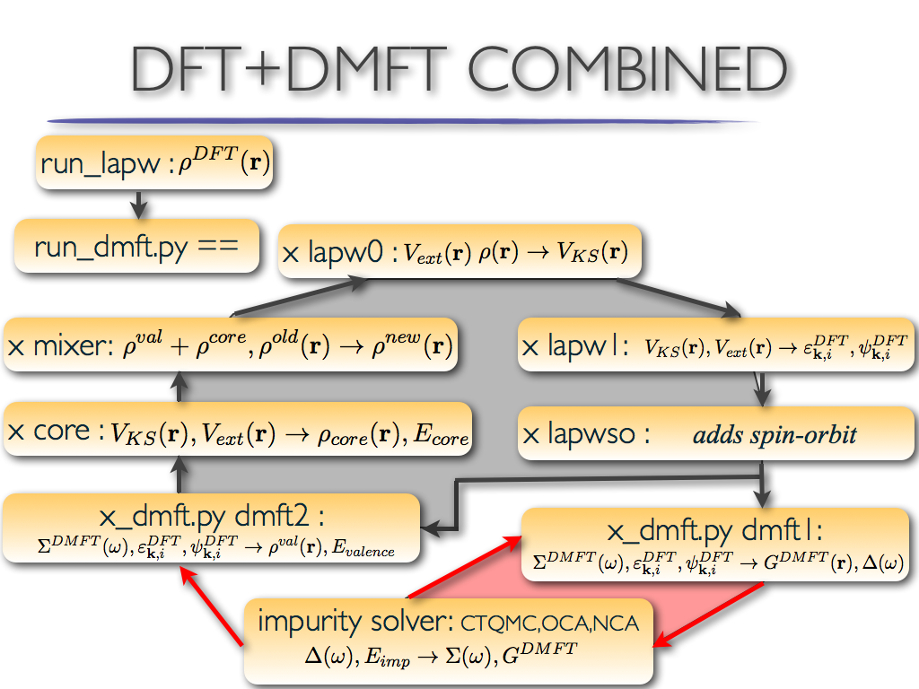
The code starts by running the lapw0 and lapw1 modules of Wien2K to calculate the vector files, etc; but then, dmft1 and dmft2 steps are inserted. Impurity is running in-between dmft1 and dmft2 step. The dmft2 step replaces the lapw2 step of Wien2k.

Since DFT part is here very fast (much faster than impurity solver), we used several DFT step (up to 100) in combination with a single dmft step. Therefore after dmft1, one can see several blocks of the following cycle repeated: dmft2,lcore,mixer,lapw0,lapw1. This is the charge loop. The reason to do this is to obtain a well converged DFT run between each dmft1 step, since dmft1 is the most time consuming part (as can be seen in the timing information above). Whether the charge density is well converged can be checked by grep'ing ':CHARGE' in the .dayfile:

grep ':CHARGE' MnO.dayfile

Which will print

:CHARGE convergence:  0.3650051
:CHARGE convergence:  0.320649
:CHARGE convergence:  0.1980197
:CHARGE convergence:  0.1882957
:CHARGE convergence:  0.1454709
:CHARGE convergence:  0.0432447
:CHARGE convergence:  0.0190978
:CHARGE convergence:  0.0055925
:CHARGE convergence:  0.0048235
:CHARGE convergence:  0.0024782
:CHARGE convergence:  0.0006552
:CHARGE convergence:  0.0001947
:CHARGE convergence:  0.0002805
:CHARGE convergence:  2.05e-05
:CHARGE convergence:  1.16e-05
:CHARGE convergence:  1.69e-05
:CHARGE convergence:  1.84e-05
:CHARGE convergence:  1.4e-06

Note that the charge converges at fixed self-energy, but when the self-energy is updated (after dmft1 step) the charge is again non-converged. Towards the end of the run (after about 20 cycles), the self enery is also converged and so the jump in the charge after each dmft1 is much less significant:

0  :CHARGE convergence: 0.3650051 
1  :CHARGE convergence: 0.320649 
2  :CHARGE convergence: 0.1980197 
3  :CHARGE convergence: 0.1882957 
4  :CHARGE convergence: 0.1454709 
5  :CHARGE convergence: 0.0432447 
6  :CHARGE convergence: 0.0190978 
7  :CHARGE convergence: 0.0055925 
8  :CHARGE convergence: 0.0048235 
9  :CHARGE convergence: 0.0024782 
10 :CHARGE convergence: 0.0006552 
11 :CHARGE convergence: 0.0001947 
12 :CHARGE convergence: 0.0002805 
13 :CHARGE convergence: 2.05e-05 
14 :CHARGE convergence: 1.16e-05 
15 :CHARGE convergence: 1.69e-05 
16 :CHARGE convergence: 1.84e-05 
17 :CHARGE convergence: 1.4e-06 
  ....
  ....
51 :CHARGE convergence: 0.0046878 
52 :CHARGE convergence: 0.0041113 
53 :CHARGE convergence: 0.00243 
54 :CHARGE convergence: 0.0013541 
55 :CHARGE convergence: 0.0006717 
56 :CHARGE convergence: 0.000342 
57 :CHARGE convergence: 0.0001287 
58 :CHARGE convergence: 3.47e-05 
59 :CHARGE convergence: 1.37e-05 
60 :CHARGE convergence: 3.6e-06 
61 :CHARGE convergence: 0.002555 
62 :CHARGE convergence: 0.0022443 
63 :CHARGE convergence: 0.0013392 
64 :CHARGE convergence: 0.0007663 
65 :CHARGE convergence: 0.0003645 
66 :CHARGE convergence: 0.0002563 
67 :CHARGE convergence: 7.28e-05 
68 :CHARGE convergence: 1.09e-05 
69 :CHARGE convergence: 9.6e-06 
70 :CHARGE convergence: 6.1e-06 
71 :CHARGE convergence: 6e-07
....
....
135 :CHARGE convergence: 0.0002954 
136 :CHARGE convergence: 0.0002592 
137 :CHARGE convergence: 0.0001538 
138 :CHARGE convergence: 0.0001346 
139 :CHARGE convergence: 5.24e-05 
140 :CHARGE convergence: 2.72e-05 
141 :CHARGE convergence: 6.8e-06 
142 :CHARGE convergence: 3.2e-06 
143 :CHARGE convergence: 0.0003925 
144 :CHARGE convergence: 0.0003348 
145 :CHARGE convergence: 0.0001878 
146 :CHARGE convergence: 0.0001563 
147 :CHARGE convergence: 4.16e-05 
148 :CHARGE convergence: 2.61e-05 
149 :CHARGE convergence: 1.05e-05 
150 :CHARGE convergence: 2.8e-06

Another important file to check is the info.iterate, which contains information about the chemical potential, the number of electrons on the V ion, etc:

  #   #.   #           mu          Vdc            Etot     Ftot+T*Simp     Ftot+T*Simp       n_latt        n_imp      Eimp[0]     Eimp[-1] 
  0   0.   0     6.531263    37.772879    -2467.797924    -2467.812926    -2467.796784     4.832377     5.013534     0.054065    -0.045105 
  1   0.   1     6.531263    37.772879    -2467.795198    -2467.839362    -2467.794737     4.856478     5.013534     0.054065    -0.045105 
  2   0.   2     6.531263    37.772879    -2467.790068    -2467.919012    -2467.791341     4.928763     5.013534     0.054065    -0.045105 
  3   0.   3     6.531263    37.772879    -2467.805037    -2468.148462    -2467.807211     5.119680     5.013534     0.054065    -0.045105 
  4   0.   4     6.531263    37.772879    -2467.806312    -2468.041367    -2467.803524     4.975357     5.013534     0.054065    -0.045105 
  5   0.   5     6.531263    37.772879    -2467.797455    -2468.058270    -2467.797604     4.989835     5.013534     0.054065    -0.045105 
  6   0.   6     6.531263    37.772879    -2467.795467    -2468.037324    -2467.795559     4.964081     5.013534     0.054065    -0.045105 
  7   0.   7     6.531263    37.772879    -2467.795670    -2468.039345    -2467.795727     4.967218     5.013534     0.054065    -0.045105 
  8   0.   8     6.531263    37.772879    -2467.795453    -2468.037709    -2467.795553     4.968465     5.013534     0.054065    -0.045105 
  9   0.   9     6.531263    37.772879    -2467.795395    -2468.034744    -2467.795412     4.970982     5.013534     0.054065    -0.045105 
 10   0.  10     6.531263    37.772879    -2467.794961    -2468.029487    -2467.794965     4.974418     5.013534     0.054065    -0.045105 
 11   0.  11     6.531263    37.772879    -2467.794815    -2468.027650    -2467.794804     4.974379     5.013534     0.054065    -0.045105 
 12   0.  12     6.531263    37.772879    -2467.794816    -2468.027676    -2467.794805     4.974472     5.013534     0.054065    -0.045105 
 13   0.  13     6.531263    37.772879    -2467.794813    -2468.027656    -2467.794803     4.974440     5.013534     0.054065    -0.045105 
 14   0.  14     6.531263    37.772879    -2467.794813    -2468.027658    -2467.794803     4.974441     5.013534     0.054065    -0.045105 
 15   0.  15     6.531263    37.772879    -2467.794813    -2468.027657    -2467.794803     4.974440     5.013534     0.054065    -0.045105 
 16   0.  16     6.531263    37.772879    -2467.794813    -2468.027655    -2467.794803     4.974440     5.013534     0.054065    -0.045105 
 17   1.   0     6.531263    37.940316    -2467.791665    -2467.796323    -2467.793875     5.101315     5.033536    -0.240213    -0.362603 
 18   1.   1     6.531263    37.940316    -2467.791016    -2467.781532    -2467.792627     5.089714     5.033536    -0.240213    -0.362603 
 19   1.   2     6.531263    37.940316    -2467.789431    -2467.737004    -2467.789185     5.054946     5.033536    -0.240213    -0.362603 
 20   1.   3     6.531263    37.940316    -2467.787966    -2467.669527    -2467.784865     5.006160     5.033536    -0.240213    -0.362603 
 21   1.   4     6.531263    37.940316    -2467.786916    -2467.648442    -2467.783808     5.018529     5.033536    -0.240213    -0.362603 
 22   1.   5     6.531263    37.940316    -2467.785769    -2467.646216    -2467.783363     5.028555     5.033536    -0.240213    -0.362603 
 23   1.   6     6.531263    37.940316    -2467.785657    -2467.641236    -2467.783057     5.024862     5.033536    -0.240213    -0.362603 
 24   1.   7     6.531263    37.940316    -2467.785486    -2467.638166    -2467.782886     5.025596     5.033536    -0.240213    -0.362603 
 25   1.   8     6.531263    37.940316    -2467.785492    -2467.638303    -2467.782892     5.025582     5.033536    -0.240213    -0.362603 
 26   1.   9     6.531263    37.940316    -2467.785489    -2467.638261    -2467.782888     5.025539     5.033536    -0.240213    -0.362603 
 27   1.  10     6.531263    37.940316    -2467.785488    -2467.638250    -2467.782887     5.025538     5.033536    -0.240213    -0.362603 
 28   1.  11     6.531263    37.940316    -2467.785489    -2467.638264    -2467.782888     5.025541     5.033536    -0.240213    -0.362603 
 29   2.   0     6.531263    37.919732    -2467.784434    -2467.789381    -2467.784203     5.024368     5.031140    -0.077242    -0.205319 
 30   2.   1     6.531263    37.919732    -2467.784453    -2467.790595    -2467.784272     5.025296     5.031140    -0.077242    -0.205319 
 31   2.   2     6.531263    37.919732    -2467.784511    -2467.794236    -2467.784480     5.028077     5.031140    -0.077242    -0.205319 
....
....
153  14.   6     6.531263    37.919319    -2467.784809    -2467.786146    -2467.784766     5.031462     5.031090    -0.090639    -0.218392 
154  14.   7     6.531263    37.919319    -2467.784806    -2467.786104    -2467.784764     5.031478     5.031090    -0.090639    -0.218392 
155  14.   8     6.531263    37.919319    -2467.784806    -2467.786091    -2467.784763     5.031482     5.031090    -0.090639    -0.218392 
156  14.   9     6.531263    37.919319    -2467.784805    -2467.786087    -2467.784763     5.031482     5.031090    -0.090639    -0.218392 
157  15.   0     6.531263    37.917886    -2467.784779    -2467.789688    -2467.784788     5.031145     5.030921    -0.085861    -0.213710 
158  15.   1     6.531263    37.917886    -2467.784780    -2467.789750    -2467.784791     5.031194     5.030921    -0.085861    -0.213710 
159  15.   2     6.531263    37.917886    -2467.784784    -2467.789936    -2467.784802     5.031343     5.030921    -0.085861    -0.213710 
160  15.   3     6.531263    37.917886    -2467.784789    -2467.790227    -2467.784820     5.031569     5.030921    -0.085861    -0.213710 
161  15.   4     6.531263    37.917886    -2467.784792    -2467.790226    -2467.784820     5.031496     5.030921    -0.085861    -0.213710 
162  15.   5     6.531263    37.917886    -2467.784793    -2467.790225    -2467.784820     5.031493     5.030921    -0.085861    -0.213710 
163  15.   6     6.531263    37.917886    -2467.784793    -2467.790227    -2467.784821     5.031488     5.030921    -0.085861    -0.213710 
164  15.   7     6.531263    37.917886    -2467.784794    -2467.790230    -2467.784821     5.031487     5.030921    -0.085861    -0.213710

The second column counts the number of DMFT steps (impurity solver), the third counts charge steps at each DMFT steps, next columns shows the chemical potential, the fifth column shows the double-counting potential, the sixth column shows total energy, followed by two different estimates of the free energy. The seventh column estimate of the free energy is not precise, instead the eight column should be used. [Notice that all quantities, except the total energy and the free energy are give in eV. The total energies and free energies are give in Ry, to be compatible with wien2k]. The ninth and tenth column show the impurity occupation computed from the solid (n_latt) and from the impurity (n_imp). The last two columns show the impurity levels.

The chemical potential in this insulating materials is fixed. The impurity occupation, computed from the solid, is quite off at the beginning, however, it becomes close to nominal 5.0 is just a few iterations. When the calculation is converged, n_latt and n_imp should match.

Very many steps appear in info.iterate file, and sometimes we just want to print one line per each dmft steps (the step at which the charge is converged, and just before the self-energy is updated). This would correspond to step 16,28,... in the above example.
We can execute

analizeInfo.py

to list only these dmft steps. We can then plot the lattice and impurity occupation, which should look like this:

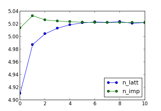Within 6 dmft iterations, the charge is converged to 5.032, and we can now increase the precision of the Monte Carlo steps. For example, increase M in params.dat file for factor of 4-5 to have much more precise statistics in the last few iterations.

Notice that each variable in params.dat file can be changed during the run, and it will be updated during the run.

Within 10 or so dmft iterations (around 120 charge iterations), the total energy and the free energy are converged within 1meV (using 216 cores for impurity solver), as seen here:

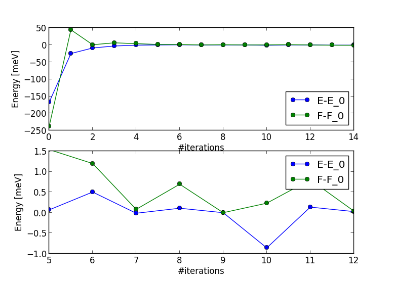Notice that total energy (or free energy) would converge better only if Monte Carlo statistics is increase, as resulting noise is due to MC noise.

Other files to monitor the run include

dmft_info.out      -- prints what is being executed, and what were parameters
MnO.scf                -- like in dft, contains energies and forces and lots of other info
dmft1_info.out         -- progress of dmft1 step
MnO.outputdmf1         -- log file of the dmft1 step. Contains the density matrix in :NCOR and the matrix of impurity levels.
dmft2_info.out         -- progress of dmft2 step
MnO.outputdmf2         -- log file of the dmft2 step (similar to MnO.output2 from lapw2); contains energies and forces.
MnO.dlt1*              -- the hybridization function
MnO.gc1*               -- the local green's function
imp.0/ctqmc.log*       -- log file of the impurity solver
imp.0/nohup_imp.out.xxx -- progress of the impurity solver for each mpi process
Delta.inp*             -- input hybridization function
imp.0/histogram.dat    -- the histogram of the perturbation order, i.e., how many kinks does the time evolution contain

Even though the impurity occupations and total energy converged, we should check the spectral functions to decide if the run is properly converged. In a metal, it is best to look at the self-energy (impurity self-energies are at : imp.0/Sig.out*, while the lattice self-energy, which is just a combination of impurity ones, are at: sig.inp*).
In a Mott insulator, the self-energy on real axis has a pole inside the gap, and therefore its shape on imaginary axis is very sensitive to the relative position of the chemical potential an the pole. If one accidentally hits the pole by placing mu on it, the self-energy on imaginary axis diverges at zero frequency. If however the chemical potential is slightly moved away from the pole, self-energy just becomes large at finite frequencies, but its imaginary part vanishes at zero. This is because on real axis the imaginary part vanishes inside the gap, except for the pole. The real part is large, but not diverging, except when chemical potential is at the pole. The shape of the self-energy on imaginary axis is therefore not very illustrative.

We will therefore rather concentrate on the Green's function, of which the imaginary part needs to vanish at zero frequency (both on the real and the imaginary axis). Here is the plot of the impurity Green's function with iterations:

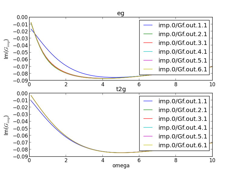We see that the green's function is metallic only at the first iteration, while at the second iteration is almost converged. Such rapid convergence is here due to the robustness of the gap in the high-spin state on Mn.

We should always check that the impurity and the local green's function of the solid match. This is a very non-trivial check of the correctness of the calculation, as the algorithm equates only the self-energy at each iteration, while the Green's functions differ until the self-consistency is achieved. We see that at the six-th dmft iteration, the two Green's functions match very well:

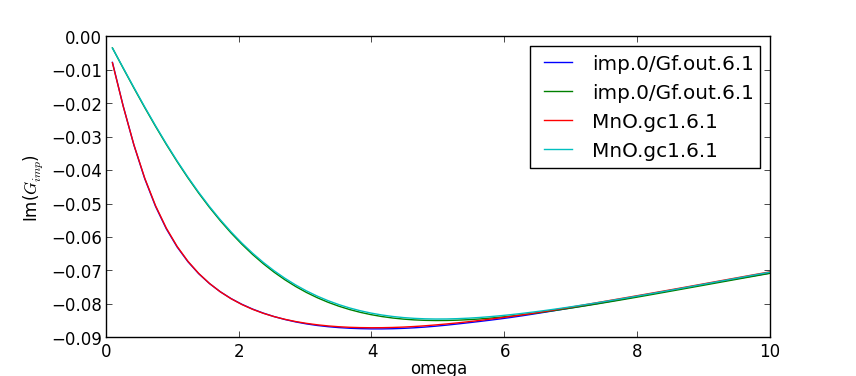Notice that the last Green's functions are named imp.0/Gf.out and MnO.gc1, while each previous iteration is saved under the same name, with consecutive number attached to it. The first number stands for the number of the outside loop, while the second number enumerates the steps inside the dmft loop (red loop in the figure above). Since we have max_dmft_iterations=1, the second number is always 1. The first number would go from 1 to the parameter finish from params.dat file, or less, if the convergence is achieved earlier

We see that for practical purposes, the convergence is achieved around 6-7th iteration, and the next steps are within the statistical noise identical. The job would not finish though, because by default (to be cautious) the convergence criteria are set very high. It is therefore desirable to kill the job, once the overal convergence is obviously achieved.

Tutorial 1.d. : Postprocessing, analytic continuation, DOS

At this point, we can proceed to the next step of plotting spectra on the real axis.

Once the calculation is done on the imaginary axis, we need to do analytical continuation to obtain the self energy on the real axis. For this, we first take average of the sig.inp files from the last few steps (in order to reduce the noise) by

saverage.py sig.inp.1[0-5].1

The output is written to sig.inpx. We could append -o option, if we wanted to change this name. All python scripts include a short help, so by executing for example

saverage.py --help

it prints the options for this script.

Next, create a new directory (lets call it maxent), and copy the averaged self energy sig.inpx into it. Also copy the maxent_params.dat file, which contains the parameters for the analytical continuation process:

params={'statistics': 'fermi', # fermi/bose
        'Ntau'      : 300,     # Number of time points
        'L'         : 20.0,    # cutoff frequency on real axis
        'x0'        : 0.005,   # low energy cut-off
        'bwdth'     : 0.004,   # smoothing width
        'Nw'        : 300,     # number of frequency points on real axis
        'gwidth'    : 2*15.0,  # width of gaussian
        'idg'       : 1,       # error scheme: idg=1 -> sigma=deltag ; idg=0 -> sigma=deltag*G(tau)
        'deltag'    : 0.004,   # error
        'Asteps'    : 4000,    # anealing steps
        'alpha0'    : 1000,    # starting alpha
        'min_ratio' : 0.001,   # condition to finish, what should be the ratio
        'iflat'     : 1,       # iflat=0 : constant model, iflat=1 : gaussian of width gwidth, iflat=2 : input using file model$
        'Nitt'      : 1000,    # maximum number of outside iterations
        'Nr'        : 0,       # number of smoothing runs
        'Nf'        : 40,      # to perform inverse Fourier, high frequency limit is computed from the last Nf points
  }

Perhaps the most important is mesh on the real axis, which is given by the upper cutoff L, the low energy cutoff x0 and Nw points. The mesh is non-uniform and more dense at low energy (tan-mesh). The MC error is here set to 0.004, and can be estimated from the variation in sig.inp.? files. Notice that we do not continue the self-energy, which would have very large error, and would not be stable to continue analytically. We will analytically continue an auxiliary function, which is constructed as

and then perform Kramers-Kronig on imaginary part of this function:

and finally invert it to solve for the self-energy on the real axis

The script which does that is called maxent_run.py. We will thus run

maxent_run.py sig.inpx

which uses the maximum entropy method to do analytical continuation. This creates the self energy Sig.out on the real axis. It should be similar to this plot:

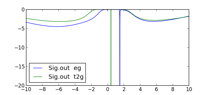Notice that both orbitals have Mott-type gap, as there is a pole in the gap. The sizes of the two gaps are different, with the eg orbitals having somewhat larger (4.8eV) and t2g smaller (2.7eV) gap.

Now we need to make one last dmft1 calculation in order to obtain the Green's function and DOS on the real axis. Create a new directory inside your output directory, and while it the new directory, use

dmft_copy.py ../

to copy necessary files from the output of the DMFT run to the new directory. Also copy the analytically continued self energy Sig.out to sig.inp in this new directory:

cp ../maxent/Sig.out sig.inp

Since we need to run the code on the real axis, we need to change the NiO.indmfl file. The first number on the second line of NiO.indmfl file determines whether the code is run on the real axis (0) or the imaginary axis (1). Change it to 0. The header of MnO.indmfl file should now look like

5 15 1 5                              # hybridization band index nemin and nemax, renormalize for interstitials, projection type
0 0.025 0.025 200 -3.000000 1.000000  # matsubara, broadening-corr, broadening-noncorr, nomega, omega_min, omega_max (in eV)
1                                     # number of correlated atoms
1     1   0                           # iatom, nL, locrot
  2   7   1                           # L, qsplit, cix

Then, inside the new directory run

x lapw0 -f  MnO
x_dmft.py lapw1
x_dmft.py dmft1

Before you might want to set OMP_NUM_THREADS to a large number (but smaller then the number of cores on your node), such as 10, to parallelize some loops with open_mp.

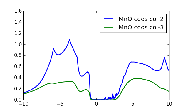
Once the run is done, we now have the densities of states on the real axis. Both the total (column 2) and partial Mn-d (column 3) are stored in MnO.cdos:

To obtain this plot, we increased the number of k-points to 10,000. The procedure is the same as above: rerun x kgen -f MnO and when asked enter 10000. Then rerun lapw1 and dmft1 step.
Notice that the first excitation into the valence band has roughly 1/3 of d-character, and 2/3 of the oxygen character. Notice also that this is not the real lower Hubbard band within our description, as U is too large (9eV). This peak is than due to screening of the Mn large spin by oxygen degrees of freedom, and is a type of Kondo effect. It is interesting to point out that even in an insulator the Kondo effect is not completely absent, as such screening occurs at the first possible excitation. In literature, such effect is also called Zhang-Rice singlet, as it was first discussed in cuprates by Zhang & Rice.

Lets note that the first excitation into the conduction band is of itinerant character, mostly 4s character, hence the scattering rate for this state is very small, and this state has very high mobility despite the correlated nature of the gap. Due to finite k-point mesh, this DOS appears somewhat spiky.

We can also take a look at the imaginary part of the green's function. Recall that the imaginary part of the green's function, divided by -pi, gives the DOS. So, plotting the even-numbered columns in the MnO.gc1 one, we can get the DOS of individual d orbitals (eg and t2g). The plot is

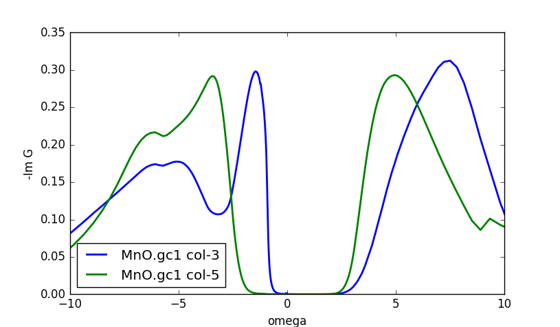Notice that column 3 is the eg, and column 5 the t2g DOS. In this plot it is even more clear that the lower Hubbard band is below -4eV, and that the first valence excitation of the eg-states is split away, making a singlet between the oxygen states and the two eg orbitals. Notice that it is exactly this type of screening (hybridization screening) which reduces the low energy Coulomb interaction, and therefore if one simulates a Hubbard model for MnO, one needs to take much smaller U. Within our embedded method, the Coulomb repulsion will thus always be large compared to model calculations, as such screening very efficiently reduces interaction in the solid.

Note that the imaginary part of green's function and DOS use slightly different normalization, therefore the sum of all green's functions will typically produce slightly larger DOS than is computed in case.cdos. This is because Green's functions are computed with normalized projectors within a mufin-thin sphere (the integral of spectral function is by construction exactly unity), while partial dos usually uses unnormalized projector.

Another quantity of physical interest is the impurity hybridization function. It is stored in the file MnO.dlt1, and its imaginary part, which has the units of eV, looks like the following:

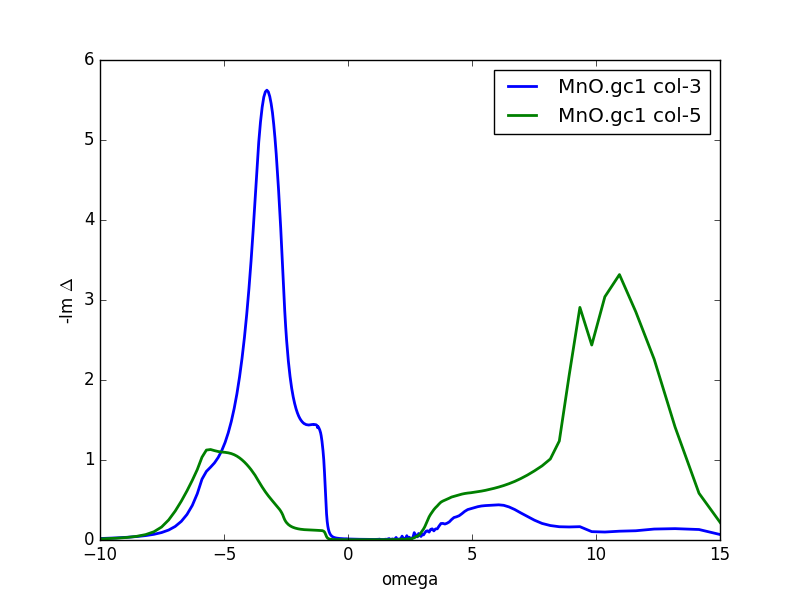
The large peak below the Fermi level signals the hybridization of eg states with the oxygen p states, as expected on the basis of previous discussion.