Two particle vertex in CTQMC

The two particle vertex in our CTQMC is computed by sampling the Fourier transform of the $M$ matrix (which is the inverse of the hybridization matrix), or, (in the newer version) it can be projected to the SVD basis functions.

Many details of our implementation are available in Hyowon Park's thesis (thesis). See Equations 4.11 - 4.13.

Here we just provide a quick summary.

We defined the two particle object by:

\begin{eqnarray} \chi_{i_0,i_1,i_2,i_3}(\nu_1,\nu_2,\Omega) = \int_0^\beta e^{i\nu_1\tau_e^1+i(\nu_2-\Omega)\tau_e^2-\nu_2\tau_s^2-i(\nu_1-\Omega)\tau_s^1 } \langle T_\tau \psi_{i_0}^\dagger(\tau_e^1)\psi_{i_1}^\dagger(\tau_e^2)\psi_{i_2}(\tau_s^2)\psi_{i_3}(\tau_s^1)\rangle \end{eqnarray}

Here index $i$ denotes the bath index, which we block diagonalize. (In general, we have index $i$ to denote the block, and internal index $b$ to denote the entry in the block, i.e., $i = (i,b)$.)

The two contributions computed by the CTQMC are:

\begin{eqnarray} \chi_{i_0,i_1,i_2,i_3}(\nu_1,\nu_2,\Omega) =\delta_{i_1 i_2}\delta_{i_0 i_3}\int_0^\beta e^{i\nu_1\tau_e^1+i(\nu_2-\Omega)\tau_e^2-\nu_2\tau_s^2-i(\nu_1-\Omega)\tau_s^1 } \langle T_\tau \psi_{i_0}^\dagger(\tau_e^1)\psi_{i_1}^\dagger(\tau_e^2)\psi_{i_1}(\tau_s^2)\psi_{i_0}(\tau_s^1)\rangle \\ +\delta_{i_0 i_2}\delta_{i_1 i_3}\int_0^\beta e^{i\nu_1\tau_e^1+i(\nu_2-\Omega)\tau_e^2-\nu_2\tau_s^2-i(\nu_1-\Omega)\tau_s^1 } \langle T_\tau \psi_{i_0}^\dagger(\tau_e^1)\psi_{i_1}^\dagger(\tau_e^2)\psi_{i_0}(\tau_s^2)\psi_{i_1}(\tau_s^1)\rangle \end{eqnarray}

Here $i$ is not just a single bath, bath can mean a matrix of possibilities.

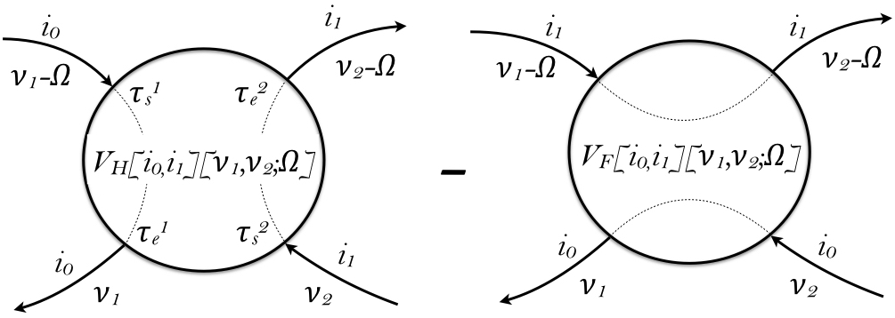
Using Feynman diagrams, we can express this object in terms of two contributions, which we call the Hartree $V_H$ and Fock $V_F$ term, depicted by:

First, we can define the two frequency object $M_{i}(\nu_1,\nu_2)$, which is (when SVD sampling is turned off) computed directly in Matsubara frequency space

\begin{eqnarray} M_{i}(\nu_1,\nu_2) = \frac{1}{\beta}\sum_{\tau_s,\tau_e}e^{i\nu_1\tau_e}M_{i}(\tau_e,\tau_s)e^{-i\nu_2\tau_s} \end{eqnarray}

This is the same object as needed for measuring the Green's function, except that Green's function corresponds to the part in which $\nu_1=\nu_2$. Hence, measuring this quantity does not cost much overhead. We here used index $i$ to denote the block of baths in which this $M$ is calculated. Note that the baths, which are not coupled, form independent matrices $M_i$.

Once we compute this $M$ object, we can construct the two parts of the two particle vertex by (derivation requires one to take the second derivative of the partition function with respect to the hybridization $\frac{\delta^2 logZ}{\delta\Delta_{i_0 i_3}\delta\Delta_{i_1 i_2}}$ -- see Hyowon's thesis above):

\begin{eqnarray} V_H[i_0,i_1][\nu_1,\nu_2;\Omega] = M_{i_0}(\nu_1,\nu_1-\Omega)\; M_{i_1}(\nu_2-\Omega,\nu_2)\\ V_F[i_0,i_1][\nu_1,\nu_2;\Omega] = M_{i_0}(\nu_1,\nu_2) \; M_{i_1}(\nu_2-\Omega,\nu_1-\Omega) \end{eqnarray}

The two particle Green's function then can be constructed by:

\begin{eqnarray} \chi_{i_0,i_1,i_2,i_3}(\nu_1,\nu_2,\Omega) = V_H[i_0,i_1][\nu_1,\nu_2;\Omega]\delta_{i_0,i_3}\delta_{i_1,i_2} - V_F[i_0,i_1][\nu_1,\nu_2;\Omega]\delta_{i_1,i_3}\delta_{i_0,i_2} \end{eqnarray}

This does not require much time, as $M(\nu_1,\nu_2)$ is already computed and stored.

These two objects ($V_H$ and $V_F$) are printed into tvertex.dat file.

Looking at the definition of $V_F$, we see that if sufficient number of Matsubara frequencies are available, $V_F$ can be computed from $V_H$ in the following way:

\begin{eqnarray} V_F[i_0,i_1][\nu_1,\nu_2;\Omega] = V_H[i_0,i_1][\nu_1,\nu_1-\Omega;\nu_1-\nu_2] \end{eqnarray}

The same algorithm is also implemented when the "SVD" basis (svd_lmax>0) is used (see paper by Shinaoka Hiroshi).