GW for electron gas
Step1 : Exchange part, the potential energy, and the $\Phi$ functional
We will calculate self-energy and $\Phi$ function for electron gas, interacting with the screened Coulomb repulsion of the form $$v(r)=\frac{e^{-\lambda r}}{4\pi\varepsilon\varepsilon_0 r}\rightarrow v_q=\frac{8\pi}{\varepsilon(q^2+\lambda^2)}$$
Exchange part
We will first calculate the exchange term. It takes the form: $$\Sigma_x(k) = -\int \frac{d^3q}{(2\pi)^3} n_q v_{k-q}=-\int_0^{k_F}\frac{ 2\pi q^2 dq}{8\pi^3\varepsilon}\int_{-1}^1 dx \frac{8\pi}{(k^2+q^2+2 k q x)+\lambda^2}=-\frac{2}{\pi\varepsilon}\int_0^{k_F} dq q^2\int_{-1}^1\frac{dx}{k^2+q^2+\lambda^2+2 k q\,x}$$
Here are some useful integrals which we will use several times: \begin{eqnarray} &&\int_{-1}^1\frac{dx}{a-b x+i\delta}=\frac{1}{b}\log\left(\frac{a+b+i\delta}{a-b+i\delta}\right) \ &&\int_0^{k_F} dk\, k [\log(a+b\,k)-\log(a-b\,k)= \frac{a\, k_F}{b} + \frac{a^2-k_F^2 b^2}{2\,b^2}[\log(a-k_F\,b)-\log(a+k_F\,b)] \end{eqnarray}
Using the first integral above, we obtain \begin{eqnarray} \Sigma_x(k)=\frac{1}{\pi\varepsilon\,k}\int_0^{k_F} dq q\log\left(\frac{\lambda^2+(k-q)^2}{\lambda^2+(k+q)^2}\right) \end{eqnarray}
Next we introduce new variables $x=\frac{k}{\lambda}$ and $y=\frac{q} {\lambda}$ and $x_F=\frac{k_F}{\lambda}$ to obtain \begin{eqnarray} \Sigma_x(k=\lambda x)=-\frac{\lambda}{\pi\varepsilon x}\int_0^{x_F} dy y \log\left(\frac{1+(x+y)^2}{1+(x-y)^2}\right)= -\frac{\lambda}{\varepsilon\,\pi} \left[ 2 x_F + 2\arctan(x-x_F)-2\arctan(x+x_F)-\frac{1-x^2+x_F^2}{2 x}\log\left(\frac{1+(x-x_F)^2}{1+(x+x_F)^2}\right) \right] \end{eqnarray}
We thus have \begin{eqnarray} \Sigma_x(k)=-\frac{2 k_F}{\varepsilon\,\pi} \left[ 1 + \frac{\lambda}{k_F} \arctan(\frac{k-k_F}{\lambda})-\frac{\lambda}{k_F} \arctan(\frac{k+k_F}{\lambda}) -\frac{(\lambda^2-k^2+k_F^2)}{4 k\, k_F} \log\left(\frac{\lambda^2+(k-k_F)^2}{\lambda^2+(k+k_F)^2}\right) \right] \end{eqnarray}
The implementation of this self-energy follows:
from scipy import *
def Sigma_x(EF, k, lam, eps):
    kF = sqrt(EF)
    pp = 0
    if lam>0:
        pp = lam/kF*(arctan((k+kF)/lam)-arctan((k-kF)/lam))
    qq = 1 - pp - (lam**2+kF**2-k**2)/(4*k*kF)*log((lam**2+(k-kF)**2)/(lam**2+(k+kF)**2))
    return -2*kF/(pi*eps)*qq
To get exchange energy, we need to compute \begin{eqnarray} E_x = \frac{1}{2}\rm{Tr}(\Sigma_x G)= \frac{2}{2}\int\frac{d^3 k}{(2\pi)^3} n_k \Sigma_x(k)=\frac{1}{2\pi^2}\int_0^{k_F}dk k^2 \Sigma_x(k) \end{eqnarray} where the factor of $2$ is due to spin degeneracy.
Finally, we insert the expression for $\Sigma_x(k)$ to obtain \begin{eqnarray} E_x=-\frac{\lambda^4}{2\varepsilon\,\pi^3}\int_0^{x_F} dx x^2\left[ 2 x_F + 2\arctan(x-x_F)-2\arctan(x+x_F)-\frac{1-x^2+x_F^2}{2 x}\log\left(\frac{1+(x-x_F)^2}{1+(x+x_F)^2}\right) \right] \end{eqnarray}
Integration can be carried out analytically, and takes the form: \begin{eqnarray} E_x = -\frac{\lambda^4}{2\varepsilon\,\pi^3}\left[ \frac{ x_F\, x(3 x^2+3 x_F^2-1)}{6} +\frac{2}{3}(x^3-x_F^3)\arctan(x-x_F)-\frac{2}{3}(x^3+x_F^3)\arctan(x+x_F) +\frac{1}{8}\log\left(\frac{1+(x-x_F)^2}{1+(x+x_F)^2}\right) \left( -\frac{1}{3}+x_F^2(x_F^2-2)+x^2(x^2-2 x_F^2-2) \right) \right]_0^{x_F} \end{eqnarray} which finally gives \begin{eqnarray} E_x=-\frac{\lambda^4}{2\varepsilon\,\pi^3}\left[ x_F^4-\frac{1}{6}x_F^2 -\frac{4}{3}x_F^3\arctan(2 x_F)+\frac{x_F^2+\frac{1}{12}}{2}\log(1+4 x_F^2) \right] \end{eqnarray} or equivalently \begin{eqnarray} E_x=-\frac{\lambda^4 x_F^4}{2\varepsilon\,\pi^3}\left[ 1-\frac{1}{6 x_F^2} -\frac{4}{3 x_F}\arctan(2 x_F)+ \frac{1+\frac{1}{12 x_F^2}}{2 x_F^2}\log(1+4 x_F^2) \right] \end{eqnarray}
Since the density is $$\rho=2\int\frac{d^3k}{(2\pi)^3} n_k=\frac{k_F^3}{3\pi^2}$$ and also $$\frac{1}{\rho}=\frac{4\pi r_S^3}{3},$$ we have $$k_F=\left(\frac{9\pi}{4}\right)^{1/3}\frac{1}{r_S}$$ which gives for exchange-energy density $$\varepsilon_x\equiv \frac{E_x}{\rho}$$ therefore we have \begin{eqnarray} \varepsilon_x = -\frac{3 k_F}{2\varepsilon\,\pi} f\left(\frac{k_F}{\lambda}\right) =-\frac{3}{2\varepsilon\,\pi} \left(\frac{9\pi}{4}\right)^{1/3}\frac{1}{r_S} f\left(\left(\frac{9\pi}{4}\right)^{1/3}\frac{1}{\lambda\,r_S}\right) \end{eqnarray} where \begin{equation} f(x)=1-\frac{1}{6 x^2} -\frac{4}{3 x}\arctan(2 x)+ \frac{1+\frac{1}{12 x^2}}{2 x^2}\log(1+4 x^2) \end{equation}
The implementation of this exchange energy density follows:
def EpsEx(rs,lam, eps):
    fx=1.
    if lam>0 :
        x = (9*pi/4)**(1./3.) *1./(lam*rs)
        fx = 1 - 1./(6*x**2) - 4*arctan(2*x)/(3*x) + (1.+1./(12*x**2))*log(1+4*x**2)/(2*x**2)
    return -(3./(2.*pi*eps))*(9*pi/4.)**(1./3.)/rs*fx
The Phi functional and the potential energy
The $\Phi$ functional within GW has the form: 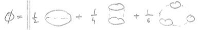 and can therefore be computes as:
The $\Phi$ functional can be summed up and becomes
\begin{eqnarray} \Phi = \frac{1}{2\beta}\sum_{q,i\Omega}\log(1-v_q P_q) \end{eqnarray}The sum over $q$ can be turned into an integral:
\begin{eqnarray} \Phi = \frac{1}{2}\int\frac{d^3q}{(2\pi)^3}\; T\sum_{i\Omega}\log(1-v_q P_q) \end{eqnarray}The self-energy within GW is:
\begin{eqnarray} \Sigma(k,i\omega)= -\frac{1}{\beta} \sum_{q,i\Omega} G(k+q,i\omega+i\Omega)\frac{v_q}{1-v_q P_{q,i\Omega}} \end{eqnarray}where the Polarization $P_{q,i\Omega}$ is
\begin{eqnarray} P_{q,i\Omega}=\frac{1}{\beta}\sum_{k,s,i\omega} G(k,i\omega) G(k+q,i\omega+i\Omega) \end{eqnarray}This can be derived directly from the Feynmann graphs.
Then the potential energy $\frac{1}{2}\rm{Tr}(\Sigma G)$ has particularly simple form:
\begin{eqnarray} E_{pot}\equiv\frac{1}{2}{\rm Tr}(\Sigma G)= -\frac{1/2}{\beta^2} \sum_{q,i\Omega,k,s,i\omega} G(k,i\omega) G(k+q,i\omega+i\Omega)\frac{v_q}{1-v_q P_{q,i\Omega}} =-\frac{1}{2\beta} \sum_{q,i\Omega} \frac{v_q P_{q,i\Omega}}{1-v_q P_{q,i\Omega}} \end{eqnarray}The Polarization
To evaluate these quantities, we thus need to calculate the polarization function $P_{q,i\Omega}$. Fortunately, if $G$ is replaced by $G^0$ (in so-called G0W0 approximation), the result can be obtained analytically.
We start by turning the fermionic $i\omega$ Matsubara sum into contour integral over the entire complex plane, but we will avoid all singularities of the product of G's:
\begin{eqnarray} P_{q,i\Omega}=-\sum_{k,s}\oint\frac{dz}{2\pi i} f(z) G(k,z)G(k+q,z+i\Omega) \equiv \sum_{k,s} p_{q,i\Omega} \end{eqnarray}This is valid because the fermi function $f(z)$ has residue equal to $-1/\beta$ in all fermionic Matsubara points, i.e., $Res(f,i\omega)=-\frac{1}{\beta}$.
In this integral, we need to avoid singularities of the Green's functions, therefore we need to integrate just above the real axis, and just below it ($z=x\pm i\delta$ with $x$ real), and we also need to cut the contour at $z=-i\Omega+x\pm i\delta$ (with $x$ real). We thus obtain:
\begin{eqnarray} p_{q,i\Omega}=-\int_{-\infty}^{\infty}\frac{dx}{\pi}f(x)\frac{1}{2i}\left[G(k,x+i\delta)-G(k,x-i\delta)\right]G(k+q,x+i\Omega) -\int_{-\infty}^{\infty}\frac{dx}{\pi}f(x-i\Omega) G(k,x-i\Omega)\frac{1}{2i}\left[G(k+q,x+i\delta)-G(k+q,x-i\delta)\right] \end{eqnarray}If we now use the form of the non-interacting $$G^0(k,x)=\frac{1}{x+\mu-\varepsilon_k},$$ we get
\begin{eqnarray} p_{q,i\Omega}=\int_{-\infty}^{\infty} dx f(x) \left[ \delta(x+\mu-\varepsilon_k) G(k+q,x+i\Omega) +G(k,x-i\Omega) \delta(x+\mu-\varepsilon_{k+q}) \right] \end{eqnarray}or, equivalently,
\begin{eqnarray} P_{q,i\Omega}= \sum_{k,s} \frac{f(\varepsilon_k-\mu)-f(\varepsilon_{k+q}-\mu)}{i\Omega+\varepsilon_k-\varepsilon_{k+q}} =2\int \frac{d^3k}{(2\pi)^3} \frac{f(\varepsilon_k-\mu)-f(\varepsilon_{k+q}-\mu)}{i\Omega+\varepsilon_k-\varepsilon_{k+q}} \end{eqnarray}Factor of 2 here is due to the spin degeneracy.
To evaluate the integral, we rewrite
\begin{eqnarray} P_{q,i\Omega}= \int \frac{dk k^2}{2\pi^2} f(\varepsilon_k-\mu) \int_{-1}^1 d(cos\theta) \left[ \frac{1}{i\Omega+\varepsilon_k-\varepsilon_{k+q}} -\frac{1}{i\Omega+\varepsilon_{k-q}-\varepsilon_k} \right] \\ =\int_0^{k_F} \frac{dk k^2}{2\pi^2} \int_{-1}^1 dx \left[ \frac{1}{i\Omega+\varepsilon(k)-\varepsilon(\sqrt{k^2+q^2+2 k q x})} -\frac{1}{i\Omega+\varepsilon(\sqrt{k^2+q^2-2 k q x})-\varepsilon(k)} \right] \end{eqnarray}We can not evaluate the integral analytically for a general dispersion $\varepsilon(k)$. However, in the LDA-type approximation (called G0W0), the potential is static and local, and depends only on $r_S$. As the density is constant in the electron gas problem, the LDA-XC potential is constant. As we work at constant density, a constant potential is exactly compensated by a constant shift in the chemical potential. Hence the Green's function within LDA approximation remains equal to the non-interacting Green's function, and hence the dispersion is not changed.
To proceed, let us intorduce dimensionless variables, $$\varepsilon(k) = \frac{\hbar^2 k^2}{2 m}=\frac{\hbar^2}{2 m a_B^2} (k a_B)^2=(k a_B)^2\; \textrm{Ry} \rightarrow k^2$$
We will measure energies in units of $\textrm{Ry}$ and lengths in units of Bohr-radius, hence $\varepsilon(k)=k^2$. The integral then becomes
\begin{eqnarray} P_{q,i\Omega}=\int_0^{k_F} \frac{dk k^2}{2\pi^2}\frac{1}{k q}\int_{|k-q|}^{k+q} du u \left( \frac{1}{i\Omega + k^2-u^2}-\frac{1}{i\Omega+u^2-k^2} \right)= \int_0^{k_F} \frac{dk k^2}{2\pi^2}\frac{1}{2 k q}\int_{(k-q)^2}^{(k+q)^2} dx \left( \frac{1}{i\Omega + k^2-x}+\frac{1}{-i\Omega+k^2-x} \right) \end{eqnarray}Next we use the integral, which we evaluated at the very top of this document, to obtain:
\begin{eqnarray} P_{q,i\Omega} = -\frac{k_F}{4\pi^2} \left[1- \frac{1}{8 k_F q}\left\{ \left[ \frac{(i\Omega-q^2)^2}{q^2}-4 k_F^2 \right] \log\left(\frac{i\Omega-q^2-2 k_F q}{i\Omega-q^2+2 k_F q}\right) + \left[ \frac{(i\Omega+q^2)^2}{q^2}-4 k_F^2 \right] \log\left(\frac{i\Omega+q^2+2 k_F q}{i\Omega+q^2-2 k_F q}\right) \right\} \right] \end{eqnarray}While this expression for polarization can be readily implemented, its evaluation is very unstable when $\Omega\gg q^2+2k_F q$. We therefore want to expand this expression, and finds its large frequency/low q limit. The expansion is standard, and is given by \begin{eqnarray} P_{q,i\Omega}(\Omega\gg q^2+2 k_F q)= -\frac{2 k_F^3}{3 \pi^2} \frac{q^2}{-(i\Omega)^2 + q^2(q^2 +\frac{12}{5} k_F^2)} \equiv \frac{c_q}{(i\Omega)^2-b_q^2} \end{eqnarray} Here we introduced: \begin{eqnarray} c_q&=&q^2\; \frac{2 k_F^3}{3 \pi^2}\ b_q&=&q \;\sqrt{q^2 +\frac{12}{5} k_F^2} \end{eqnarray}
The implementation of polarization $P_{q,i\Omega}$ on imaginary axis is provided below:
def Polarisi(q,w,EF):
    """ Polarization P(q,iW) on imaginary axis. Note that the result is real.
        It works on arrays of frequency, i.e., w can be array of bosonic Matsubara points.
    """
    kF = sqrt(EF)
    q2 = q**2
    kFq = 2*kF*q
    D = 1./(8.*kF*q)

    if type(w)==ndarray:
        res = zeros(len(w),dtype=float)

        # careful for small q or large w
        is_w_large = w > 20*(q2+kFq) # for w[i>=iw_start] we should use power expansion
        iw_start = len(w)  # if this was newer true, is_w_large contains only False => iw_start=len(w)
        if is_w_large[-1] : # If at least the last frequency is larger than the cutoff, we can find the index
            iw_start = argmax( is_w_large )

        # if w < cutoff use exact expression
        iw = w[:iw_start]*1j
        wmq2 = iw-q2
        wpq2 = iw+q2
        C1 = log(wmq2-kFq)-log(wmq2+kFq)
        C2 = log(wpq2-kFq)-log(wpq2+kFq)
        res[:iw_start] = real( -kF/(4*pi**2) * (1. - D*(wmq2**2/q**2-4*EF)*C1 + D*(wpq2**2/q**2-4*EF)*C2) )
        # if w < cutoff use proper power expansion
        b2 = q2 * ( q2 + 12./5. * EF ) # b2==b^2
        c = 2*EF*kF*q2/(3*pi**2)
        res[iw_start:] = -c/(w[iw_start:]**2 + b2)
    else:
        # careful for small q or large w
        if  w <= 20*(q2+kFq) :
            iw = w*1j
            wmq2 = iw-q2
            wpq2 = iw+q2
            C1 = log(wmq2-kFq)-log(wmq2+kFq)
            C2 = log(wpq2-kFq)-log(wpq2+kFq)
            res = real( -kF/(4*pi**2) * (1. - D*(wmq2**2/q**2-4*EF)*C1 + D*(wpq2**2/q**2-4*EF)*C2) )
        else:
            b2 = q2 * ( q2 + 12./5. * EF )
            c = 2*EF*kF*q2/(3*pi**2)
            res = -c/(w**2 + b2)
    return res
Back to Phi functional and the potential energy
The form of the $\Phi$ functional and the potential energy $E_{pot}$ was derived above:
\begin{eqnarray} \Phi &=& \frac{1}{2}\int\frac{d^3q}{(2\pi)^3}\; T\sum_{i\Omega}\log(1-v_q P_q) \\ E_{pot}&=&-\frac{1}{2} \int\frac{d^3q}{(2\pi)^3} T\sum_{i\Omega} \frac{v_q P_{q,i\Omega}}{1-v_q P_{q,i\Omega}} \end{eqnarray}We will now implement only the correlation part, as the exchange was already computed above more efficiently (and analytically). Both terms contain, at the lowest order, the same exchange part
\begin{equation} E_x=-\frac{1}{2}\int \frac{d^3q}{(2\pi)^3} T \sum_{i\Omega} v_q P_q \end{equation}which we will take out.
We thus have
\begin{eqnarray} \Phi^c &=& \frac{1}{4\pi^2}\int_0^\infty dq\; q^2\; T\sum_{i\Omega}\left(\log(1-v_q P_q)+v_q P_q\right) \\ E_{pot}^c &=&\frac{1}{4\pi^2} \int_0^\infty dq\; q^2\; T\sum_{i\Omega} \left(-\frac{v_q P_{q,i\Omega}}{1-v_q P_{q,i\Omega}}+v_q P_q\right) \end{eqnarray}Matsubara mesh
But before we start summing over Matsubara points, we need to invent an efficient mesh for Matsubara points. We usually need several thousand Matsubara points, which can not be all evaluated. A stardard solution is to create a low frequency, and a high frequency mesh. The first usually contains all Matsubara points within very limited interval, and the second is logarithmic over large energy scale. Here we will do something different. We will construct a mesh, which is a hybrid between linear and cubic mesh, which is linear at low frequency, and becomes gradually cubic at high frequency. The implementation is here:
def GivePolyMesh(x0,L,Nw,power=3,negative=True):
    """ polynomial mesh of the type
        mesh = a * x + b * x**power
        where x=[-1,1] with 2*Nw+1 points (including zero)
        and a and b are determed by x0 & L.
        Requires : x0 > L/Nw**power
                    L > Nw*x0
    """

    den = 1-1./Nw**(power-1)
    alpha = (Nw*x0 - L/Nw**(power-1))/den
    beta = (L - Nw*x0)/den
    if negative:
        x = linspace(-1,1,2*Nw+1)
    else:
        x = linspace(0,1,Nw+1)
    om = alpha*x + beta*x**power
    return om
Here we test such mesh using 50 points instead of 1000 points.
from pylab import *
# Import Bokeh modules for interactive plotting
import bokeh.io
import bokeh.mpl
import bokeh.plotting
# Magic function to make matplotlib inline; other style specs must come AFTER
%matplotlib inline
#%matplotlib notebook
# This enables SVG graphics inline.  There is a bug, so uncomment if it works.
%config InlineBackend.figure_formats = {'svg',}
# This enables high resolution PNGs. SVG is preferred, but has problems
# rendering vertical and horizontal lines
# %config InlineBackend.figure_formats = {'png', 'retina'}
# Set up Bokeh for inline viewing
bokeh.io.output_notebook()

msh = [round(x) for x in GivePolyMesh(1,1000,50,negative=False)]
semilogy(msh[1:],'o-')
show()
print msh
Once we have an efficient method to sum over Matsubara points, we will implement the following Matsubara sums:
\begin{eqnarray} Sq_1(q)=T\sum_{i\Omega}\left(\log(1-v_q P_q)+v_q P_q\right)\\ Sq_2(q)=T\sum_{i\Omega} \left(-\frac{v_q P_{q,i\Omega}}{1-v_q P_{q,i\Omega}}+v_q P_q\right) \end{eqnarray}from scipy import interpolate
def Phi_Functional_inside(beta, EF, q, lam, eps, plt=False):
"""computes the Phi functional and the potential energy of
electron gas within G0W0 approximation.
"""
def GiveLimits(M_max):
"Returns the value of the function at this Matsubara point"
Wm = M_max*2*pi*T
Pq = Polarisi(q,Wm,EF)
return abs(log(1-vq*Pq) + vq*Pq)
T=1./beta
kF = sqrt(EF)
vq = 8*pi/(eps*(q**2+lam**2))
# First we compute how many Matsubara points is needed
M_max = 1000 # First start with 1000 points.
limits = GiveLimits(M_max) # How small is the function at this frequency?
if limits > 1e-6: # The value is larger than 1e-6. We want to increase M.
while ( limits > 1e-6 and M_max>50):
M_max = int(M_max*1.2)
limits = GiveLimits(M_max)
elif limits < 1e-7: # The value is too small. We can safely decrease M.
while (limits < 1e-7 and M_max>50):
M_max = int(M_max/1.2)
limits = GiveLimits(M_max)
else:
pass
Nw_max=100 # Number of frequencies in non-uniform mesh
M_max = max(M_max, Nw_max) # The number of all Matsubara points should always be larger than those in poly mesh.
M_max = min(M_max, Nw_max**3-1) # and should be smaller than M**3, because we use cubic mesh.
# Produces non-uniform mesh of formula y = a*x + b*x^3, which a and b choosen such that the first
# few points have distance 1 (0,1,...) and we have in total M_max~100 points extended up to M_max~1000.
Wm_small = array([round(x) for x in GivePolyMesh(1.,M_max,Nw_max,3,False)])
Wm_small *= 2*pi*T # small bosonic Matsubara mesh prepared
Pq = Polarisi(q,Wm_small,EF) # Now we evaluate Polarization on this mesh of ~100 points
Sq_x = -vq*Pq # Exchange part
# Phi functional withouth exchange part
Sq1 = log(1-vq*Pq) - Sq_x # We keep only correlation part, because exchange part does not converge in this formula
# 1/2*Tr(Sigma*G) part withouth exchange part
Sq2 = Sq_x/(1+Sq_x) - Sq_x # We keep only correlation part, because exchange part does not converge in this formula
Wm = 2*pi*T*arange(0,M_max+1) # All Matsubara points up to cutoff (~1000 points)
# We now interpolate on the entire mesh, using information from the smaller poly mesh.
Sq1_tot = interpolate.UnivariateSpline(Wm_small, real(Sq1), s=0)(Wm)
# And now we just perform the sum. The zero point is special in bosonic case. The rest of the points appear twice.
phi = T*( Sq1_tot[0] + 2*sum(Sq1_tot[1:]) )
# We also interpolate the potential energy.
Sq2_tot = interpolate.UnivariateSpline(Wm_small, real(Sq2), s=0)(Wm)
trSG2 = T*( Sq2_tot[0] + 2*sum(Sq2_tot[1:]) )
if plt:
plot(Wm_small/(2*pi*T), -Sq1, 'o-')
plot(Wm/(2*pi*T), -Sq1_tot, '-')
xlim([0,100])
show()
return array([phi, trSG2])
Let's check the quality of Matsubara interpolation:
%matplotlib inline
from pylab import *
Phi_Functional_inside(beta=100, EF=1.0, q=0.5, lam=0, eps=1, plt=True)
And finaly we compute the two quantities by integration over momentum
\begin{eqnarray} \Phi^c &=& \frac{1}{4\pi^2}\int_0^\infty dq\; q^2\; Sq_1(q) \\ E_{pot}^c &=&\frac{1}{4\pi^2} \int_0^\infty dq\; q^2\; Sq_2(q) \end{eqnarray}from scipy import integrate
def Phi_Functional(beta, EF, lam, eps, plt=False):
kF = sqrt(EF)
rho = kF**3/(3*pi**2)
qs = linspace(1e-6, 6*kF,2**7+1) # reasonable q-mesh with 129 points
phis = array([Phi_Functional_inside(beta, EF, q, lam, eps,plt=False)*q**2 for q in qs])
Phi = integrate.romb(phis[:,0], dx=qs[1]-qs[0])/(4*pi**2)
trSG2 = integrate.romb(phis[:,1], dx=qs[1]-qs[0])/(4*pi**2)
if plt:
plot(qs, phis[:,0], 'o-',label='Phi')
plot(qs, phis[:,1], 's-',label='trSG2')
legend(loc='best')
show()
return (Phi/rho,trSG2/rho)
%matplotlib inline
Phi_Functional(beta=100, EF=1., lam=0,eps=1,plt=True)
LDA correlation energy
Next we code one of the standard LDA parametrizations for the exchange-correlation energy:
class  ExchangeCorrelation:
    """*************************************************************************/
    Calculates Exchange&Correlation Energy and Potential                       */
             S.H.Vosko, L.Wilk, and M.Nusair, Can.J.Phys.58, 1200 (1980)       */
    ****************************************************************************/
    """
    def __init__(self):
        self.alphax = 0.610887057710857 #//(3/(2 Pi))^(2/3)
        self.Ap  =  0.0621814
        self.xp0 = -0.10498
        self.bp  =  3.72744
        self.cp  =  12.9352
        self.Qp  =  6.1519908
        self.cp1 =  1.2117833
        self.cp2 =  1.1435257
        self.cp3 = -0.031167608

    def Vx(self, rs): # Vx
        return -2*self.alphax/rs

    def ExVx(self, rs): # Ex-Vx
        return 0.5*self.alphax/rs

    def Ex(self, rs):
        return -1.5*self.alphax/rs

    def Vc(self, rs): # Vc
        x=sqrt(rs)
        xpx= x*x + self.bp*x + self.cp
        atnp = arctan(self.Qp/(2*x+self.bp))
        ecp = 0.5*self.Ap*(log(x*x/xpx)+self.cp1*atnp-self.cp3*(log((x-self.xp0)**2/xpx)+self.cp2*atnp))
        return 2*(ecp - self.Ap/6.*(self.cp*(x-self.xp0)-self.bp*x*self.xp0)/((x-self.xp0)*xpx))

    def EcVc(self, rs): # Ec-Vc
        x = sqrt(rs)
        return 2*(self.Ap/6.*(self.cp*(x-self.xp0)-self.bp*x*self.xp0)/((x-self.xp0)*(x*x+self.bp*x+self.cp)))
Now we put together the $\Phi$ functional, potential energy, and the LDA correlation energy:
%matplotlib inline
def test():
    exc=ExchangeCorrelation()
    CF = (9*pi/4.)**(1./3.)
    rs = linspace(0.5,8,20)
    EC = zeros(len(rs))
    Phi = zeros(len(rs))
    trSG2 = zeros(len(rs))
    for i, rs0 in enumerate(rs):
        kF = CF/rs0
        EF = kF**2
        (Phi[i], trSG2[i]) = Phi_Functional(beta=100, EF=EF, lam=0, eps=1)
        EC[i] = exc.EcVc(rs0) + exc.Vc(rs0)
    plot(rs,EC, label='EC_LDA')
    plot(rs, Phi, label='Phi')
    plot(rs, trSG2, label='1/2Tr(SG)')
    plot(rs, (Phi-2*trSG2)/(-1), label='-(Phi-Tr(SG))')
    #plot(rs, Phi/1.5, label='Phi/1.5')
    plot(rs, (Phi+trSG2)/4,label='(Phi+Epot)/4')
    legend(loc='best')
test()
Step 2: The correlation self-energy
The self-energy is given by:
\begin{eqnarray} \Sigma(k,i\omega)=-\frac{1}{\beta}\sum_{q,i\Omega} G(k+q,i\omega+i\Omega)\frac{v_q}{1-v_q P_{q,i\Omega}} \end{eqnarray}We first split it into exchange and the correlation part:
\begin{eqnarray} &&\Sigma^x(k,i\omega)=-\frac{1}{\beta}\sum_{q,i\Omega} G(k+q,i\omega+i\Omega)v_q\\ &&\Sigma^c(k,i\omega)=-\frac{1}{\beta}\sum_{q,i\Omega} G(k+q,i\omega+i\Omega)\left(\frac{v_q}{1-v_q P_{q,i\Omega}}-v_q\right) \end{eqnarray}Next we turn the sum into the integral over momentum $q$
\begin{eqnarray} \Sigma^c(k,i\omega)= -\int\frac{d^3q}{(2\pi)^3}\; T\sum_{i\Omega}G(k+q,i\omega+i\Omega)\left(\frac{v_q}{1-v_q P_q}-v_q\right) \end{eqnarray}and then split it into the integral over the angle and the modulus of $q$:
\begin{eqnarray} \Sigma^c(k,i\omega)= -\frac{1}{4\pi^2}\int dq\; q^2 \; T\sum_{i\Omega}\left(\frac{v_q}{1-v_q P_q}-v_q\right) \int_{-1}^1 dx \frac{1}{i\omega+i\Omega+\mu-\varepsilon(\sqrt{k^2+q^2+2kqx})} \end{eqnarray}Within G0W0 the Green's function is not changed from the non-interacting $G^0$, therefore $\varepsilon(k)=k^2$, and we can evaluate the innermost integral analytically:
We split this evaluation into sum over frequency, and integral over momentum:
\begin{eqnarray} &&R(k,i\omega,q)\equiv\frac{1}{2kq}\; T\sum_{i\Omega} \left(\frac{1}{1-v_q P_q}-1\right) \log\left(\frac{i\omega+i\Omega+E_F-(k-q)^2}{i\omega+i\Omega+E_F-(k+q)^2}\right) \\ &&\Sigma^c(k,i\omega)=-\frac{1}{4\pi^2}\int dq\; q^2 \; v_q\; R(k,i\omega,q) \end{eqnarray}At large frequency $\Omega$ the sum in $R$ falls off as $1/\Omega^2$. However, we can calculate even the cubic term, and we will do that here. At large $\Omega$ we have
\begin{eqnarray} \log\left(\frac{i\omega+i\Omega+E_F-(k-q)^2}{i\omega+i\Omega+E_F-(k+q)^2}\right)\approx \frac{4 k q}{i\Omega+i\omega+E_F-k^2-q^2} \equiv \frac{4 k q}{i\Omega+i\omega-\xi} \end{eqnarray}and \begin{eqnarray} \frac{1}{1-v_q P_q}-1=\frac{v_q}{\frac{1}{P_q}-v_q}\approx \frac{v_q}{\frac{(i\Omega)^2-b_q^2}{c_q}-v_q} =\frac{v_q c_q}{{(i\Omega)^2-b_q^2}-v_q c_q}=\frac{v_q c_q}{(i\Omega)^2-a_q^2} \end{eqnarray} with $$\xi=k^2+q^2-EF$$ $$a_q^2=b_q^2+v_q c_q$$
We hence see that
\begin{eqnarray} R(k,i\omega,q)\approx\frac{1}{2kq}T\sum_{i\Omega}\frac{4 k q}{i\Omega+i\omega-\xi}\frac{v_q c_q}{(i\Omega)^2-a_q^2} ={2 v_q c_q}\;T\sum_{i\Omega}\frac{1}{i\Omega+i\omega-\xi}\frac{1}{(i\Omega)^2-a_q^2} \end{eqnarray}We will now define
\begin{eqnarray} && R_\infty \equiv {2 v_q c_q}\;T\sum_{i\Omega}\frac{1}{i\Omega+i\omega-\xi}\frac{1}{(i\Omega)^2-a_q^2}\\ && R_0\equiv T\sum_{i\Omega}\frac{1}{i\Omega+i\omega-\xi}\frac{1}{(i\Omega)^2-a_q^2} \end{eqnarray}Next we evaluate the sum \begin{eqnarray} R_0 =\oint \frac{dz}{2\pi i}n(z)\frac{1}{z+i\omega-\xi}\frac{1}{z^2-a_q^2} \end{eqnarray}
We next use the identity \begin{eqnarray} \frac{1}{z+i\omega-\xi}\frac{1}{z^2-a_q^2} =\frac{1}{2a} \left( \frac{1}{z+i\omega-\xi} \frac{1}{z-a}- \frac{1}{z+i\omega-\xi} \frac{1}{z+a} \right) \end{eqnarray}
and \begin{eqnarray} \frac{1}{z+i\omega-\xi}\frac{1}{z^2-a_q^2}= \frac{1}{2a(i\omega-\xi+a)} \left( \frac{1}{z-a}-\frac{1}{z+i\omega-\xi} \right) -\frac{1}{2a(i\omega-\xi-a)} \left( \frac{1}{z+a}-\frac{1}{z+i\omega-\xi} \right) \end{eqnarray}
therefore \begin{eqnarray} R_0=-\frac{n(a)+f(\xi)}{2a(i\omega-\xi+a)} +\frac{n(-a)+f(\xi)}{2a(i\omega-\xi-a)} =-\frac{n(a)}{2a(i\omega-\xi+a)} +\frac{n(-a)}{2a(i\omega-\xi-a)}+\frac{f(\xi)}{(i\omega-\xi-a)(i\omega-\xi+a)} \end{eqnarray}
We just obtained: \begin{eqnarray} R(k,i\omega,q)\approx R_\infty=\frac{v_q c_q}{a_q}\left(\frac{n(-a_q)+f(\xi)}{i\omega-\xi-a_q}-\frac{n(a_q)+f(\xi)}{i\omega-\xi+a_q}\right) \end{eqnarray}
To numerically evaluate $R(k,i\omega,q)$ sum, we will compute
\begin{equation} R(k,i\omega,q)= \frac{1}{2kq}\; T\sum_{i\Omega} \left(\frac{1}{1-v_q P_q}-1\right) \log\left(\frac{i\omega+i\Omega+E_F-(k-q)^2}{i\omega+i\Omega+E_F-(k+q)^2}\right)- {2 v_q c_q}\;T\sum_{i\Omega}\frac{1}{i\Omega+i\omega-\xi}\frac{1}{(i\Omega)^2-a_q^2} +R_\infty \end{equation}so that the numericall sum over $i\Omega$ can be truncated at relatively small value of $\Omega$
def n_bose(x,beta):
    if x*beta>100:
        return 0.0
    elif x*beta<-100:
        return -1.0
    else:
        return 1./(exp(x*beta)-1.)

def ferm(x,beta):
    if x*beta>100:
        return 0.0
    elif x*beta<-100:
        return 1.0
    else:
        return 1./(exp(x*beta)+1.)


def Rkwq(beta, EF, n, k, q, lam, eps, plt=False):
    """ Calculates the Matsubara sum of
       R(k,iw,q) = T*sum_{iW} (1/(1-v_q*P_q)-1) * Integrate[G(iw+iW,sqrt(k^2+q^2-2kq*cost)),{cost,-1,1}]
       At high frequency we subtract the approximation, which goes as 1/iW^3, as explained above.
    """
    def GiveLimits(M_max):
        Wm_limits = array([(-(M_max+2)-n)*2*pi*T, (M_max+2-n)*2*pi*T])
        PqW = Polarisi(q,Wm_limits,EF)
        Wwmn = (Wm_limits + wn)*1j + EF
        C1_limits = (log(Wwmn - kmq2) - log(Wwmn - kpq2))/(2*k*q) * (1./(1.-vq*PqW)-1.)
        C2_limits = -2*vq*cq/((Wwmn - k2q2)*(Wm_limits**2+aq**2))
        dC = C1_limits-C2_limits
        return sqrt(dC[0].real**2+dC[1].real**2)

    T=1./beta
    vq = 8*pi/(eps*(q**2+lam**2))
    wn = (2*n+1)*pi*T
    k2q2 = k**2+q**2

    kmq2 = (k-q)**2
    kpq2 = (k+q)**2

    bq2 = q**2 * ( q**2 + 12./5. * EF )
    kF=sqrt(EF)
    cq = 2*EF*kF*q**2/(3*pi**2)
    aq = sqrt(bq2 + vq*cq )

    small=1e-6
    M_max = int( (8./3.*k2q2/small)**(1./3.)/(2*pi*T) + n-1 )
    if M_max<50: M_max=50
    limits = GiveLimits(M_max)
    #print 'M_max=', M_max, 'limits=', limits
    if limits > 1e-4:
        while ( limits > 1e-4 and M_max>50):
            M_max = int(M_max*1.2)
            limits = GiveLimits(M_max)
            #print 'M_max=', M_max, limits
    elif limits < 1e-5:
        while (limits < 1e-5 and M_max>50 and M_max>n/2):
            M_max = int(M_max/1.2)
            limits = GiveLimits(M_max)
            #print 'M_max=', M_max, limits
    else:
        pass
    #print 'M_max=', M_max, 'limits=', limits

    #GivePolyMesh requires : x0 > L/Nw**power  and L > Nw*x0 hence
    #   M_max+1 > Nw_max
    #   M_max+1 < Nw_max**3
    Nw_max=30  # This is the number of points we actually evaluate
    M_max = max(M_max, n/2)
    M_max = max(M_max, Nw_max)
    M_max = min(M_max, Nw_max**3-1)
    Wm_small_ = [round(x) for x in GivePolyMesh(1.,M_max+1,Nw_max)]
    # Where is zero on this mesh?
    n_0 = Wm_small_.index(0)
    # Creating a combine mesh centered around 0 and around iw.
    Wm_small=[]
    for x in Wm_small_:
        if x<=n/2:
            Wm_small.append(x-n)
    for x in Wm_small_:
        if x>-n/2:
            Wm_small.append(x)

    Wm_small = array(Wm_small)*(2*pi*T)

    PqW = Polarisi(q,Wm_small,EF)
    Wwmn = (Wm_small + wn)*1j + EF
    # both frequency dependent quantities
    C1_small = (log( Wwmn - kmq2 ) - log( Wwmn - kpq2 ))/(2*k*q) * (1./(1.-vq*PqW)-1.)
    C2_small = -2*vq*cq/((Wwmn - k2q2)*(Wm_small**2+aq**2))

    # The difference needs to be interpolate on the entire mesh, to sum over Matsubara mesh
    dCrl = interpolate.UnivariateSpline(Wm_small[:n_0+1], real(C1_small[:n_0+1]-C2_small[:n_0+1]), s=0)
    dCil = interpolate.UnivariateSpline(Wm_small[:n_0+1], imag(C1_small[:n_0+1]-C2_small[:n_0+1]), s=0)
    dCrr = interpolate.UnivariateSpline(Wm_small[n_0:], real(C1_small[n_0:]-C2_small[n_0:]), s=0)
    dCir = interpolate.UnivariateSpline(Wm_small[n_0:], imag(C1_small[n_0:]-C2_small[n_0:]), s=0)
    # entire Matsubara mesh
    Wml = 2*pi*T*arange(-M_max-n-1,-n)
    Wmr = 2*pi*T*arange(-n,M_max+1)
    # Here is finally the sum over the entire Matsubara mesh
    R1 = sum(dCrl(Wml))*T + sum(dCrr(Wmr))*T + 1j*sum(dCil(Wml))*T + 1j*sum(dCir(Wmr))*T
    # We still need to add the high frequency correction
    wnkq=wn*1j+EF-k2q2
    xi=k2q2-EF
    R3 = vq*cq/aq * ((n_bose(-aq,beta)+ferm(xi,beta))/(wnkq-aq)-(n_bose(aq,beta)+ferm(xi,beta))/(wnkq+aq))

    if plt:
        print 'n=', n, 'q=', q, 'k=', k
        figure()
        plot(Wm_small/(2*pi*T), real(C1_small), 'o', label='C1.real')
        plot(Wm_small/(2*pi*T), imag(C1_small), 'o', label='C1.imag')
        plot(Wm_small/(2*pi*T), real(C1_small-C2_small), 'o', label='C1-C2.real')
        plot(Wm_small/(2*pi*T), imag(C1_small-C2_small), 'o', label='C1-C2.imag')
        plot(Wml/(2*pi*T), dCrl(Wml), '-', label='C1-C2.real')
        plot(Wml/(2*pi*T), dCil(Wml), '-', label='C1-C2.imag')
        plot(Wmr/(2*pi*T), dCrr(Wmr), '-', label='C1-C2.real')
        plot(Wmr/(2*pi*T), dCir(Wmr), '-', label='C1-C2.imag')
        legend(loc='best')
        show()

    return R1+R3
At high frequency $i\omega$ or small momentum $q$, the numeric calculation of the correlation self-energy has problems, and we want to calculate this limit analytically. We start with the above derived expansion of polarization :
\begin{eqnarray} P_{q,i\Omega}(\Omega\gg q^2+2 k_F q)= \frac{c_q}{(i\Omega)^2-b_q^2} \end{eqnarray}with \begin{eqnarray} c_q&=&q^2\; \frac{2 k_F^3}{3 \pi^2}\ b_q&=&q \;\sqrt{q^2 +\frac{12}{5} k_F^2} \end{eqnarray} and with that, we calculate the correlation self-energy
\begin{eqnarray} \widetilde{\Sigma}^c(k,i\omega)= -\int\frac{d^3q}{(2\pi)^3}\;v_q\; T\sum_{i\Omega}G(k+q,i\omega+i\Omega) \left(\frac{1}{1-v_q P_q}-1\right) \\ =-\int\frac{d^3q}{(2\pi)^3}\;v_q\; T\sum_{i\Omega} \frac{1}{i\Omega+i\omega-\xi_{k,q}} \frac{v_q c_q}{(i\Omega)^2-a_q^2} \end{eqnarray}with $$a_q^2=b_q^2+v_q c_q$$ and $$\xi_{k,q}=(\vec{k}+\vec{q})^2-\mu$$
We derived above that
\begin{eqnarray} R_0\equiv T\sum_{i\Omega}\frac{1}{i\Omega+i\omega-\xi}\frac{1}{(i\Omega)^2-a^2} =\frac{n(-a)+f(\xi)}{2a(i\omega-\xi-a)}-\frac{n(a)+f(\xi)}{2a(i\omega-\xi+a)} \end{eqnarray}so that
\begin{eqnarray} \widetilde{\Sigma}^c(k,i\omega)= -\int\frac{d^3q}{(2\pi)^3}\;\frac{v_q^2 c_q}{2 a_q}\; \left[\frac{n(-a_q)+f(\xi_{k,q})}{(i\omega-\xi_{k,q}-a_q)}-\frac{n(a_q)+f(\xi_{k,q})}{(i\omega-\xi_{k,q}+a_q)}\right] \end{eqnarray}We thus arrive at:
\begin{eqnarray} \widetilde{\Sigma}^c(k,i\omega)=-\int_0^\infty\;dq\frac{2\pi q^2}{(2\pi)^3}\;\frac{v_q^2 c_q}{2 a_q}\; \left[n(-a_q)\int_{-1}^1 dx \frac{1}{i\omega+E_F-a_q-(k^2+q^2-2 k q x)}-n(a_q)\int_{-1}^1 dx\frac{1}{i\omega+E_F+a_q-(k^2+q^2+2 k q x)}\right] \\ -\int_0^\infty\;dq\frac{2\pi q^2}{(2\pi)^3}\;\frac{v_q^2 c_q}{2 a_q}\; \int_{-1}^1 dx\; f(k^2+q^2-E_F+2 k q x)\left[\frac{1}{i\omega+E_F-a_q-(k^2+q^2+2 k q x)}-\frac{1}{i\omega+E_F+a_q-(k^2+q^2+2 k q x)}\right] \end{eqnarray}which is evaluated to
\begin{eqnarray} \widetilde{\Sigma}^c(k,i\omega)=-\int_0^\infty\;dq\frac{q^2}{4\pi^2}\;\frac{v_q^2 c_q}{4 a_q\;k q}\; \left[ {n(-a_q)} \log\left(\frac{i\omega+E_F-a_q-k^2-q^2+2 k q}{i\omega+E_F-a_q-k^2-q^2-2 k q}\right) +{n(a_q)} \log\left(\frac{i\omega+E_F+a_q-k^2-q^2-2 k q}{i\omega+E_F+a_q-k^2-q^2+2 k q}\right)\right] \\ -\int_0^\infty\;dq\frac{q^2}{4\pi^2}\;\frac{v_q^2 c_q}{2 a_q}\; \int_{-1}^1 dx\; f(k^2+q^2-E_F+2 k q x)\left[\frac{1}{i\omega+E_F-a_q-(k^2+q^2+2 k q x)}-\frac{1}{i\omega+E_F+a_q-(k^2+q^2+2 k q x)}\right] \end{eqnarray}We first split the self-energy into two parts, one which has only integral over $q$ left, and the other that requires further consideration:
\begin{eqnarray} \widetilde{\Sigma}^c(k,i\omega) \equiv \Sigma^c_1(k,i\omega)+\Sigma^c_2(k,i\omega) \end{eqnarray}\begin{eqnarray} \Sigma^c_1(k,i\omega)=-\int_0^\infty\;dq\frac{q^2}{4\pi^2}\;\frac{v_q^2 c_q}{4 a_q\;k q}\; \left[ {n(-a_q)} \log\left(\frac{i\omega+E_F-a_q-k^2-q^2+2 k q}{i\omega+E_F-a_q-k^2-q^2-2 k q}\right) +{n(a_q)} \log\left(\frac{i\omega+E_F+a_q-k^2-q^2-2 k q}{i\omega+E_F+a_q-k^2-q^2+2 k q}\right)\right] \end{eqnarray}\begin{eqnarray} \Sigma^c_2(k,i\omega)=-\int_0^\infty\;dq\frac{q^2}{4\pi^2}\;\frac{v_q^2 c_q}{2 a_q}\; Q(k,i\omega,q) \end{eqnarray}We just defined $Q(k,i\omega,q)$, which can also be evaluated analytically at T=0 (when $f(x)$ is a step function), but special attention has to be payed to the limits.
We first define: \begin{eqnarray} Q(k,i\omega,q)\equiv \int_{-1}^1 dx\; f(k^2+q^2-E_F+2 k q x)\left[\frac{1}{i\omega+E_F-a_q-(k^2+q^2+2 k q x)}-\frac{1}{i\omega+E_F+a_q-(k^2+q^2+2 k q x)}\right] \end{eqnarray}
(1) When $k^2+q^2-2 k q-E_F>0$ (or equivalently $(k-q)^2>E_F$ or $|k-q|>k_F$) there will be no contribution to the integral.
(2) When $(k-q)^2 < E_F < (k+q)^2$ the fermi function is negative between -1 and $(E_F-k^2-q^2)/(2kq)$. We thus have
\begin{eqnarray} Q(k,i\omega,q)=\theta\left(|k-q| < k_F\right)\int_{-1}^{min((E_F-k^2-q^2)/(2kq),1)} dx\;\left[\frac{1}{i\omega+E_F-a_q-(k^2+q^2+2 k q x)}-\frac{1}{i\omega+E_F+a_q-(k^2+q^2+2 k q x)}\right] \end{eqnarray}and consequently
\begin{eqnarray} Q(k,i\omega,q)=\theta\left(|k-k_F| < q < k+k_F\right)\frac{1}{2kq} \left[ \log\left(\frac{i\omega+E_F-a_q-(k-q)^2}{i\omega-a_q}\right) -\log\left(\frac{i\omega+E_F+a_q-(k-q)^2}{i\omega+a_q}\right) \right] \end{eqnarray}(3) When $E_F>(k+q)^2$, we have
\begin{eqnarray} Q(k,i\omega,q)=\theta\left(|k+q| < k_F\right)\int_{-1}^{1} dx\;\left[\frac{1}{i\omega+E_F-a_q-(k^2+q^2+2 k q x)}-\frac{1}{i\omega+E_F+a_q-(k^2+q^2+2 k q x)}\right] \end{eqnarray}This term is clearly nonzero only when $k+q
First, let us derive the case $k>k_F$:
\begin{eqnarray} \Sigma^c_2(k,i\omega)=-\int_{|k-k_F|}^{k+k_F}\;dq\frac{q^2}{4\pi^2}\;\frac{v_q^2 q^2\; \frac{2 k_F^3}{3 \pi^2}}{2 a_q}\; \frac{1}{2kq} \left[ \log\left(\frac{i\omega+E_F-a_q-(k-q)^2}{i\omega-a_q}\right) -\log\left(\frac{i\omega+E_F+a_q-(k-q)^2}{i\omega+a_q}\right) \right] \end{eqnarray}where we substututed $c_q=q^2\; \frac{2 k_F^3}{3 \pi^2}$.
The final result for $k>k_F$ is thus:
\begin{eqnarray} \Sigma^c_2(k,i\omega)=-\frac{k_F^3}{6\pi^4}\int_{|k-k_F|}^{k+k_F}\;dq\;\frac{(v_q q^2)^2}{4 a_q\; k\,q}\; \left[ \log\left(\frac{i\omega+E_F-(k-q)^2-a_q}{i\omega+E_F-(k-q)^2+a_q}\right) -\log\left(\frac{i\omega-a_q}{i\omega+a_q}\right) \right] \end{eqnarray}and for $k < k_F$ we have two terms:
\begin{eqnarray} \Sigma^c_2(k,i\omega)=-\frac{k_F^3}{6\pi^4}\int_{|k_F-k|}^{k+k_F}\;dq\;\frac{(v_q q^2)^2}{4 a_q\; k\,q}\; \left[ \log\left(\frac{i\omega+E_F-(k-q)^2-a_q}{i\omega+E_F-(k-q)^2+a_q}\right) -\log\left(\frac{i\omega-a_q}{i\omega+a_q}\right) \right] \\ -\frac{k_F^3}{6\pi^4}\int_0^{k_F-k}\;dq \;\frac{(v_q q^2)^2}{4 a_q\,k\,q}\; \left[ \log\left(\frac{i\omega+E_F-(k-q)^2-a_q}{i\omega+E_F-(k-q)^2+a_q}\right) -\log\left(\frac{i\omega+E_F-(k+q)^2-a_q}{i\omega+E_F-(k+q)^2+a_q}\right) \right] \end{eqnarray}We also want to repeat the expression for
\begin{eqnarray} \Sigma^c_1(k,i\omega)=-\frac{k_F^3}{6 \pi^4} \int_0^\infty\;dq\;\frac{(v_q q^2)^2}{4 a_q\;k\, q}\; \left[ {n(-a_q)} \log\left(\frac{i\omega+E_F-(k-q)^2-a_q}{i\omega+E_F-(k+q)^2-a_q}\right) +{n(a_q)} \log\left(\frac{i\omega+E_F-(k+q)^2+a_q}{i\omega+E_F-(k-q)^2+a_q}\right)\right] \end{eqnarray}We just managed to write $\widetilde{\Sigma}^c(k,i\omega)\equiv \Sigma^c_1(k,i\omega)+\Sigma^c_2(k,i\omega)$ as a single integral over $q$, which is relatively easy ti implement. The implementation follows below.
def Sigc_High_Frequency_or_Small_q(q, beta, EF, n, k, lam, eps):
    def GiveQDep(q):
        vq = 8*pi/(eps*(q**2+lam**2))      # v_q
        b2 = q**2 * ( q**2 + 12./5. * EF ) # b_q^2
        c = 2*kF**3*q**2/(3*pi**2)         # c_q
        a = sqrt(b2 + vq*c )               # a_q
        kmq2 = (k-q)**2
        kpq2 = (k+q)**2
        amiw = iw+EF-kmq2
        apiw = iw+EF-kpq2
        vqq = vq*q**2
        vqq2 = (vqq)**2/(4*a*k*q)
        return (vq, a, amiw, apiw, vqq, vqq2)

    kF = sqrt(EF)
    wn = (2*n+1)*pi/beta
    iw = wn*1j
    pref = kF**3/(6*pi**4)

    # cc -- correlation part
    # xx -- exchange part
    (vq, a, amiw, apiw, vqq, vqq2) = GiveQDep(q)
    # first part : -kF^3/(6*pi^4) * (v_q*q^2)^2/(4*a*k*q) * ( n(-a) * log((iw+EF-(k-q)^2-a)/(iw+EF-(k+q)^2-a)) - n(a) *  log((iw+EF-(k-q)^2+a)/(iw+EF-(k+q)^2+a)) )
    n_ma = array([n_bose(-aq,beta) for aq in a])
    n_a  = array([n_bose( aq,beta) for aq in a])
    cc = n_ma * log((amiw-a)/(apiw-a)) + n_a * log((apiw+a)/(amiw+a))
    xx = zeros(len(cc))

    if k<kF:
        for i, _q in enumerate(q):
            if _q < kF-k: # q < kF-k and k<kF
                cc[i] += log((amiw[i]-a[i])/(amiw[i]+a[i])) - log((apiw[i]-a[i])/(apiw[i]+a[i]))
                xx[i] += -vqq[i]/(pi**2) * 0.5

            elif _q < kF+k: # q is in [kF-k,kF+k] and k<kF
                cc[i] += log((amiw[i]-a[i])/(amiw[i]+a[i])) - log((iw-a[i])/(iw+a[i]))
                xx[i] += -vqq[i]/(pi**2) * (kF**2- (_q-k)**2)/(8*k*_q)
    else:
        # first part : -kF^3/(6*pi^4) * (v_q*q^2)^2/(4*a*k*q) * ( log((iw+EF-(k-q)^2-a)/(iw+EF-(k-q)^2+a)) - log((iw-a)/(iw+a)) )
        for i, _q in enumerate(q):
            if _q > k-kF and _q < k+kF: # q must satisfy : q in [k-kF, k+kF]
                cc[i] += log((amiw[i]-a[i])/(amiw[i]+a[i])) - log((iw-a[i])/(iw+a[i]))
                xx[i] += -vqq[i]/(pi**2) * (kF**2- (_q-k)**2)/(8*k*_q)
    res = -pref * vqq2 * cc #+ xx
    return res
Below we implement numerically $\Sigma^c(k,i\omega)$, which requires one integral over momentum $q$ of $R(k,i\omega,q)$, or, the $q$ integral for $\widetilde{\Sigma}^c$.
We split the $q$ integral into 4 intervals: \begin{eqnarray} [0,T], [T,|k_F-k|], [|k_F-k|,k_F+k], [k_F+k,\max(5(k+k_F),8k_F)] \end{eqnarray} because the function tends to have discontinuous derivative at those points.
def Sigma_c(beta, EF, n, k, lam, eps, plt=False):
    """Numeric calculation of Sigma_correlation"""
    kF = sqrt(EF)

    lowest_point = 1./beta
    kend = max(kF+k+0.5,min( 5*(kF+k), 8*kF))

    if k>0.1:
        ab = sort( [lowest_point, abs(kF-k) ] )
        lowest_point = ab[0]
        qxs= [linspace(ab[0], ab[1], 2**4+1 ),
              linspace(ab[1], kF+k,  2**6+1),
              linspace(kF+k, kend, 2**5+1 )]
    else:
        dk = min(0.05,kF/2.)
        qxs = [linspace(lowest_point, abs(kF-k)-dk, 2**4+1 ),
               linspace(abs(kF-k)-dk, kF+k+dk,  2**6+1 ),
               linspace(kF+k+dk, kend, 2**5+1 )]

    res=0
    # Very small q should be computed analytically
    qx = linspace(1e-6,lowest_point,2**2+1)

    cc2 = Sigc_High_Frequency_or_Small_q(qx, beta, EF, n, k, lam, eps)
    res += integrate.romb(cc2,dx=qx[1]-qx[0])

    if plt:
        plot(qx, real(cc2)*(-pi/2), 's-', label='Re: mesh -1')
        plot(qx, imag(cc2)*(-pi/2), 's-', label='Im: mesh -1')

    max_val=-1e100
    # The rest of the points computed numerically
    for ii,qx in enumerate(qxs):
        cc = array([Rkwq(beta, EF, n, k, q, lam, eps) * q**2/(eps*(q**2+lam**2)) for q in qx])
        max_val = max(max_val, max(abs(cc)) )
        res += -2/pi*integrate.romb(cc,dx=qx[1]-qx[0])
        if plt:
            plot(qx, real(cc), 'o-', label='Re: mesh '+str(ii))
            plot(qx, imag(cc), 'o-', label='Im: mesh '+str(ii))

    # Sometimes the range of q-integration is not sufficient, and q-points beyond kend contribute.
    # This seems to happen most often when lambda is large.
    val = abs(cc[-1])
    value_at_the_end = val/max_val
    if value_at_the_end > 1e-2: # we need to extend the q-mesh
        q = qxs[-1][-1]
        while val/max_val > 1e-2:
            q *= 2.
            v = Rkwq(beta, EF, n, k, q, lam, eps) * q**2/(eps*(q**2+lam**2))
            val = abs(v)
        #print 'Found how far we need to go ', q, qx[-1], val/max_val
        qx2 = linspace(qxs[-1][-1],q,2**5+1)
        cc2 = array([Rkwq(beta, EF, n, k, q, lam, eps) * q**2/(eps*(q**2+lam**2)) for q in qx2])
        res += -2/pi*integrate.romb(cc2,dx=qx2[1]-qx2[0])

        if plt:
            plot(qx2, real(cc2), 'o-', label='Re: mesh '+str(ii))
            plot(qx2, imag(cc2), 'o-', label='Im: mesh '+str(ii))

    if plt:
        legend(loc='best')
        grid()
        show()
    return res
Here we compute the approximation for the self-energy, as defined in the above equation $\widetilde{\Sigma_c}$
def Sigma_c_high_w(beta, EF, n, k, lam, eps, plt=False):
    """Calculation of Sigma_correlation for high frequency"""
    kF = sqrt(EF)
    lowest_point = 1./beta
    kend = max(kF+k+0.5,min( 5*(kF+k), 8*kF))
    if k>0.1:
        ab = sort( [lowest_point, abs(kF-k) ] )
        lowest_point = ab[0]
        qxs= [linspace(1e-6,lowest_point,2**2+1),
              linspace(ab[0], ab[1], 2**4+1 ),
              linspace(ab[1], kF+k,  2**6+1),
              linspace(kF+k, kend, 2**5+1 )]
    else:
        dk = min(0.05,kF/2.)
        qxs = [linspace(1e-6,lowest_point,2**2+1),
               linspace(lowest_point, abs(kF-k)-dk, 2**4+1 ),
               linspace(abs(kF-k)-dk, kF+k+dk,  2**6+1 ),
               linspace(kF+k+dk, kend, 2**5+1 )]

    res=0
    max_val = -1e100
    for ii,qx in enumerate(qxs):
        cc = Sigc_High_Frequency_or_Small_q(qx, beta, EF, n, k, lam, eps)
        max_val = max(max_val, max(abs(cc)) )
        res += integrate.romb(cc,dx=qx[1]-qx[0])
        if plt:
            plot(qx, real(cc)*(-pi/2), 'o-', label='Re: mesh '+str(ii))
            plot(qx, imag(cc)*(-pi/2), 'o-', label='Im: mesh '+str(ii))

    # Sometimes the q-mesh extnding to kend is not sufficient.
    val = abs(cc[-1])
    value_at_the_end = val/max_val
    if value_at_the_end > 1e-2: # we need to extend the q-mesh
        q = qxs[-1][-1]
        while val/max_val > 1e-2:
            q *= 2.
            v = Sigc_High_Frequency_or_Small_q(array([q]), beta, EF, n, k, lam, eps)[-1]
            val = abs(v)
        #print 'Found how far we need to go ', q, qx[-1], val/max_val
        qx2 = linspace(qxs[-1][-1],q,2**5+1)
        cc2 = Sigc_High_Frequency_or_Small_q(qx2, beta, EF, n, k, lam, eps)
        res += integrate.romb(cc2,dx=qx2[1]-qx2[0])

        if plt:
            plot(qx2, real(cc2)*(-pi/2), 'o-', label='Re: mesh '+str(ii))
            plot(qx2, imag(cc2)*(-pi/2), 'o-', label='Im: mesh '+str(ii))

    if plt:
        legend(loc='best')
        grid()
        show()
    return res
The code below generates 2D mesh in (i$\omega$,k) space and computes $\Sigma_c$ on that mesh, and saves it to a file
mesh\_rs\_+str(rs)+.datand
SigC\_rs\_+str(rs)+.dat
def Compute_and_Save_SigmaC(rs, lam, eps, beta=100., nom_low=40, nom_high=40, nom_max=10000):
    "Computes Sigma_c on a 2D mesh of k,iw, and saves it to SigC_rs_xx.dat, mesh_rs_xx.dat"
    def Give2DMesh(EF, beta, nom_low=40, nom_high=40, nom_max=10000):
        " Gives k,iw mesh"
        kF=sqrt(EF)
        # Mesh for variable k
        km = hstack( ([1e-10], linspace(0.01,0.9*kF, 10), linspace(0.9*kF,1.2333*kF, 20)[1:], linspace(1.2333*kF, 2.1*kF, 5)[1:]) )
        # cutoff of Matsubara frequency treated numerically
        n_cutoff = int( (round((sqrt(kF)*100*beta)/pi)-1)/2 )
        nw1 = array([int(round(x)) for x in GivePolyMesh(1.,n_cutoff,nom_low-1,3,False)])
        # Second Matsubara mesh computed analytically in the range [n_cutoff, nom_max+n_cutoff] with nom points
        nw2 = array([int(round(x))+nw1[-1] for x in GivePolyMesh(nw1[-1]-nw1[-2],nom_max,nom_high-1,3,False)])
        nw = hstack( (nw1, nw2[1:]) )
        return (nw, km)

    CF = (9*pi/4.)**(1./3.)
    kF = CF/rs
    EF=kF**2

    # LDA exchange correlation
    exc=ExchangeCorrelation()
    EC_LDA = exc.EcVc(rs) + exc.Vc(rs)
    # G0W0 parts of the functional
    (Phi, trSG2) = Phi_Functional(beta=beta, EF=EF, lam=lam, eps=eps)

    (nw, km) = Give2DMesh(EF, beta=beta, nom_low=nom_low, nom_high=nom_high, nom_max=nom_max)
    headertxt = '%d %d %d  %f %f %f %f  %f %f %f # Nw,Nk,nom_low, kF,beta,lam,eps, PhiC,EpotC0,EC_LDA' % (len(nw),len(km), nom_low, kF, beta, lam, eps, Phi, trSG2, EC_LDA)
    end = '_rs_'+str(rs)+'_eps_'+str(eps)+'_lam_'+str(lam)+'.dat'
    savetxt('mesh'+end, hstack( (nw, km) ).transpose(), header=headertxt)
    SigC_all = zeros( (len(km),len(nw)), dtype=complex )
    for ik,k in enumerate(km):
        SigC =  [Sigma_c(beta, EF, n, k, lam=lam,eps=eps) for n in nw[:nom_low]]
        SigCH = [Sigma_c_high_w(beta, EF, n, k, lam=lam,eps=eps) for n in nw[nom_low:]]
        SigC_ = SigC+SigCH # concatanating the low and high frequency part
        SigC_all[ik,:] = array(SigC_) # saving it
    savetxt('SigC'+end, SigC_all.view(float).T)
The cell below will take approximately 4 minutes to evaluate.
rsx=[1,2]
for rs in rsx:
    Compute_and_Save_SigmaC(rs=rs, lam=0, eps=1, beta=100.)
print 'Finished'
Now we preapre to read the compute self-energy. First the mesh
def ReadMesh(fmesh):
    dat = loadtxt(fmesh).transpose()
    fi = open(fmesh,'r')
    firstline = fi.readline()[1:].split()

    N_w, N_k, nom_low = map(int, firstline[:3])
    (kF, beta, lam, eps) = map(float, firstline[3:7])
    (PhiC,EpotC0,EC_LDA) = map(float, firstline[7:10])
    fi.close()
    nw = dat[:N_w]
    km = dat[N_w:]
    return (nw, km, nom_low, kF, beta, lam, eps)
And below we read self-energy with the mesh. Now we can plot it in any direction.
rs=2
eps0=1
lam0=0
end = '_rs_'+str(rs)+'_eps_'+str(eps0)+'_lam_'+str(lam0)+'.dat'
(nw, km, nom_low, kF, beta, lam, eps) = ReadMesh('work/mesh'+end)
SigC_all = loadtxt('work/SigC'+end)
SigC_all = SigC_all[::2,:] + SigC_all[1::2,:]*1j
%matplotlib inline

for ik in range(0,len(km),10):
    plot(nw, real(SigC_all[:,ik]), 'o-', label='real k=%4.2f'%km[ik])
    plot(nw, imag(SigC_all[:,ik]), 's-', label='imag k=%4.2f'%km[ik])
legend(loc='best')
xlim([0,200])
show()
%matplotlib inline

for iw in range(0,10,3):
    plot(km, real(SigC_all[iw,:]), 'o-', label='real nw='+str(int(nw[iw])))
    plot(km, imag(SigC_all[iw,:]), 's-', label='imag nw='+str(int(nw[iw])))
legend(loc='best')
show()
The complete code, whit parallel mpi execution, is available here.